Download as PDF, PPTX
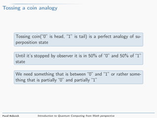
![SWAP gate
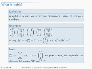
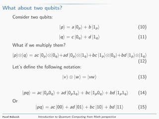
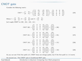
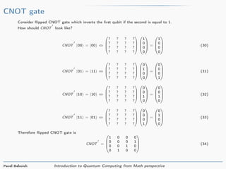
What if we apply CNOT, flipped CNOT and CNOT consequently?
Figure: SWAP circuit [I. Chuang(2004b)]
SWAP =
1 0 0 0
0 1 0 0
0 0 0 1
0 0 1 0
1 0 0 0
0 0 0 1
0 0 1 0
0 1 0 0
1 0 0 0
0 1 0 0
0 0 0 1
0 0 1 0
=
1 0 0 0
0 0 1 0
0 1 0 0
0 0 0 1
(35)
Pavel Belevich Introduction to Quantum Computing from Math perspective](https://image.slidesharecdn.com/introductiontoquantumcomputingfrommathperspective-180328145845/85/Introduction-to-Quantum-Computing-from-Math-perspective-19-320.jpg)
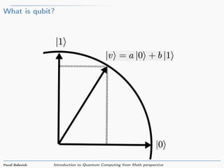
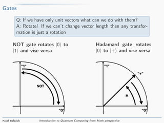
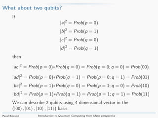
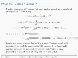
![Creating Bell state
Consider two qubits and let’s apply H to the first and CNOT to both:
Figure: EPR Creation [I. Chuang(2004a)]
CNOT(H ⊗ I) |00 =
1 0 0 0
0 1 0 0
0 0 0 1
0 0 1 0
1
√
2
1 1
1 −1
⊗
1 0
0 1
1
0
0
0
=
1
√
2
1 0 0 0
0 1 0 0
0 0 0 1
0 0 1 0
1 0 1 0
0 1 0 1
1 0 −1 0
0 1 0 −1
1
0
0
0
=
1
√
2
1
0
0
1
=
1
√
2
1
0
0
0
+
0
0
0
1
=
1
√
2
(|00 + |11 )
Pavel Belevich Introduction to Quantum Computing from Math perspective](https://image.slidesharecdn.com/introductiontoquantumcomputingfrommathperspective-180328145845/85/Introduction-to-Quantum-Computing-from-Math-perspective-21-320.jpg)

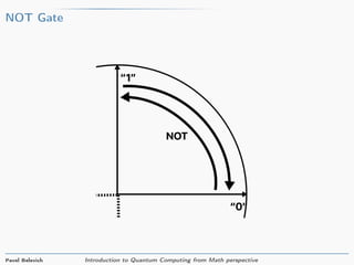
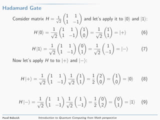
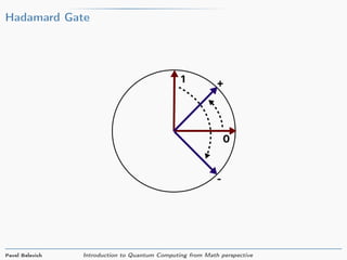
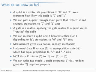
The document provides an introduction to quantum computing from a mathematical perspective. It defines a qubit as a unit vector in a two-dimensional complex vector space. Common qubit states like |0⟩ and |1⟩ are described. Basic quantum gates like the Hadamard gate and NOT gate are introduced as matrices that rotate qubit states. The document explains that two qubits can be represented as a four-dimensional vector and describes how gates like CNOT operate on multi-qubit states. In summary, the document introduces the basic mathematical concepts underlying quantum computing including qubit states, gates as rotations, and representations of multi-qubit systems.


![Polymer [ बहुलक ] Chemistry Notes PDF - Irfanullah Mehar - JJ Sir Chemistry.pdf](https://cdn.slidesharecdn.com/ss_thumbnails/polymerchemistrynotespdf-irfanullahmehar-jjsirchemistry-260210172118-3f9b37f7-thumbnail.jpg?width=640&height=640&fit=bounds)


