Description of normal distribution

1. Introduction to
Normal Distribution
The normal distribution is a fundamental concept in
statistics. It describes a bell-shaped curve that
represents the distribution of many natural
phenomena.
RUFI SHAIKH

2. Definition and Properties
1 Continuous
Distribution
The normal distribution is
a continuous probability
distribution. This means
that any value within the
range of the distribution is
possible.
2 Symmetrical
The curve is symmetrical
around its mean, which
represents the central
tendency of the data.
3 Unimodal
The curve has a single peak,
representing the most
frequent value in the data
set.
4 Empirical Rule
Approximately 68%, 95%,
and 99.7% of the data falls
within 1, 2, and 3 standard
deviations from the mean,
respectively.

3. Bell-Shaped Curve
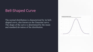
The normal distribution is characterized by its bell-
shaped curve, also known as the Gaussian curve.
The shape of the curve is determined by the mean
and standard deviation of the distribution.

4. Standard Deviation
The standard deviation is a measure of how spread
out the data is. A larger standard deviation indicates
greater variability in the data.

5. Applications of Normal Distribution
Quality Control
The normal distribution is used to monitor and
control the quality of products in manufacturing
processes.
Finance
It is used to model the returns of financial assets,
such as stocks and bonds, and to assess risk.
Social Sciences
It is used to study social phenomena, such as
intelligence, personality, and attitudes.
Healthcare
It is used to analyze patient data, such as blood
pressure and cholesterol levels.

6. Practical Examples and
Interpretations
Heights of Adults
The heights of adult men and women in a population are
often modeled by a normal distribution.
IQ Scores
Intelligence quotient (IQ) scores are standardized to follow
a normal distribution with a mean of 100 and a standard
deviation of 15.
Blood Pressure
Blood pressure readings are also commonly distributed
normally, and deviations from the norm can indicate health
concerns.

7. Density Function
In statistics, a density function refers to a mathematical
function that describes the likelihood of a continuous
random variable taking on a particular value.
A density function helps us understand how likely certain
outcomes are

8. Standardization
Standardization (or z-score normalization) is a process in
statistics used to transform data so that it has a mean of 0
and a standard deviation of 1. This transformation allows
you to compare data from different distributions or scales by
putting them on a common scale.
Uses of SNV(0,1)
1. Simplifies Calculation – no worry about
different means or sd
2. Comparison of datasets
3. Universal Reference – One universal set
of table
Where:
•Z is the z-score (standardized value),
•X is the original data point,
•μ is the mean of the data,
•σ is the standard deviation of the data.

9. Example
Imagine you have two students:
•Student A scored 85 on an exam where the mean score was 75
with a sd of 10.
•Student B scored 1900 on a standardized test where the mean
was 1500 with a standard deviation of 400.
Standardized Score
Student A - 1
Student B - 1
Both students are 1 standard deviation above the mean for their
respective tests, meaning their relative performance compared to
others is similar, despite different scales.
Standardization converts data
to a common scale by removing
the mean and scaling to unit
variance. This makes it easier to
compare and analyze data from
different sources or distributions.

10. Page 45
Example 1:
X is weight of sleep
μ = 198 gm and σ = 13 gm
Z score
Conclusion:175 gm is likely normal, as it falls within the typical range of variation.230 gm is likely
abnormal, as it is more than 2 standard deviations away from the mean

11. Page 45
Example 3:

12. Confidence Interval
A confidence interval (CI) in statistics is a range of values,
derived from a sample, that is likely to contain the true
population parameter (e.g., mean, proportion, or risk) with a
specified level of confidence.
Most commonly used is 95%
Where:
•μ is the mean,
•σ is the standard deviation,
•n is the sample size (if known, we will assume n is
large),
•Z is the Z-score corresponding to the desired confidence
level. For a 95% CI, the Z-score is approximately 1.96.

13. Example
Imagine you have two students:
•Student A scored 85 on an exam where the mean score was 75 with a sd of 10.
•Student B scored 1900 on a standardized test where the mean was 1500 with a
standard deviation of 400.
Assume n =49
95% CI
Student A - [72.2, 77.8]
Student B - [1388, 1612]
These intervals give us a range of values in which we are 95% confident the
true population means for Student A's and Student B's scores fall.

14. Standard Error
Measures how much variability exists in a sample mean
relative to the true population mean. It tells us how much
the sample mean (like the average score in a group of
students) is expected to fluctuate if we were to repeat the
sampling process multiple times.
Student A – 1.43
Student B – 57.14

15. Margin of Error
represents the amount added to and subtracted from the
sample mean to create the confidence interval. It reflects
the maximum expected difference between the sample
mean and the true population mean with a certain level of
confidence (typically 95%)
Student A – 2.8
Student B – 112
The margin of error for Student B is
112, which means the confidence
interval around the sample mean is
extended by 112 points in both
directions (giving the range 1388 to
1612)
MOE depends on SE.
Both quantity help in quantifying precision and uncertainty of
our sample estimates