Download to read offline

![Introduction to Functional Languages
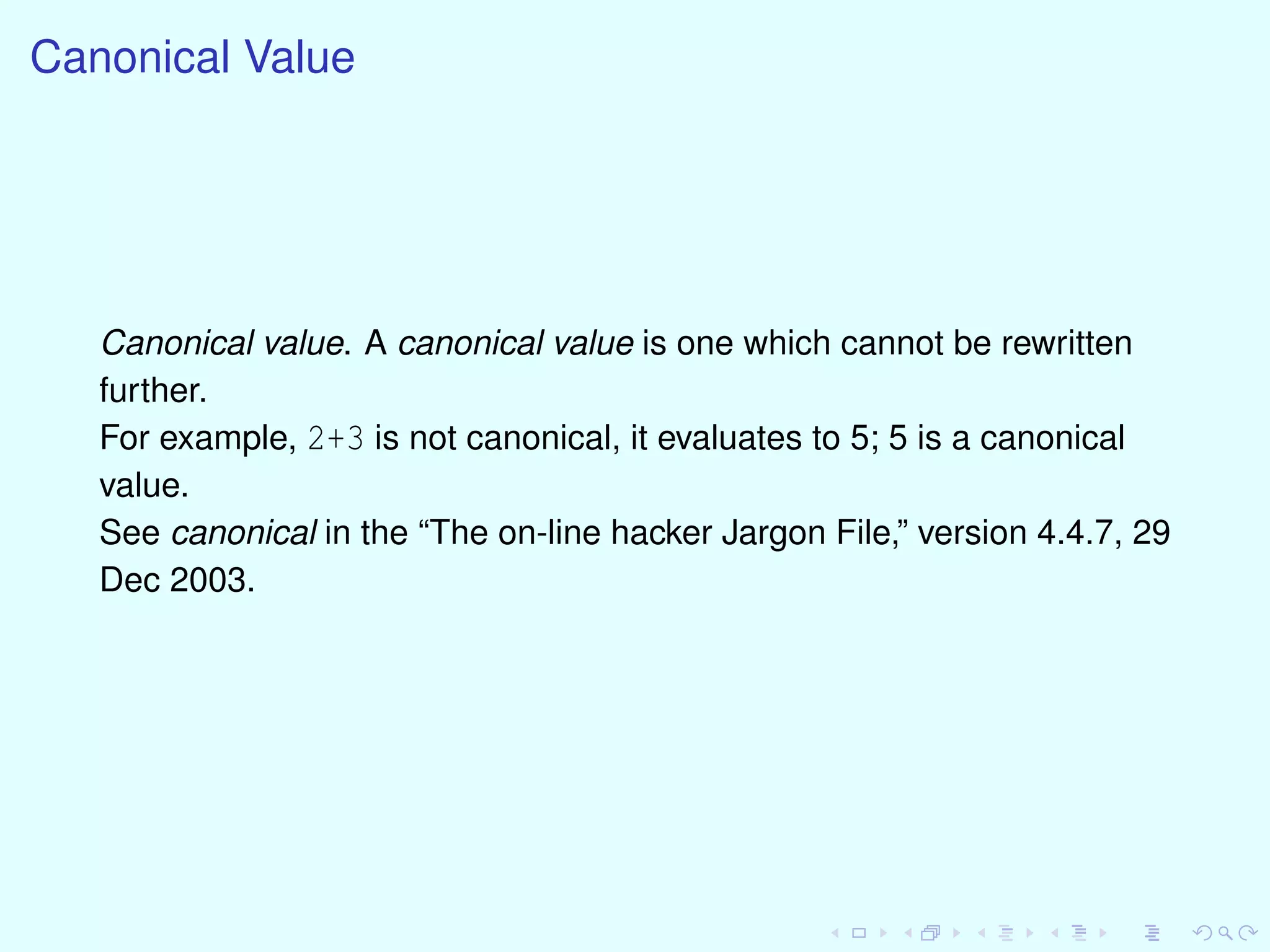
1. Referential transparency, no side effects
“substitution of equals for equals”
2. Function definitions can be used
Suppose f is defined to be the function (fn x=>exp), then f
(arg) can be replaced by exp[x := arg]
3. Lists not arrays
4. Recursion not iteration
5. Higher-order functions
New idioms, total procedural abstraction](https://image.slidesharecdn.com/fun-151224070521/75/Introduction-to-Functional-Languages-2-2048.jpg)
![Rewriting
fun square x = x * x;
fun sos (x,y) = (square x) + (square y);
sos (3,4)
==> (square 3) + (square 4) [Def’n of sos]
==> 3*3 + (square 4) [Def’n of square]
==> 9 + (square 4) [Def’n of *]
==> 9 + 4*4 [Def’n of square]
==> 9 + 16 [Def’n of *]
==> 25 [Def’n of +]
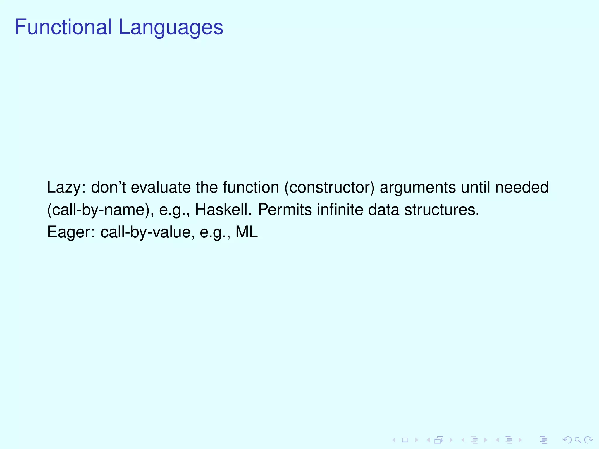
Language of expressions only, no statements.
fun test (x) = if x>20 then "big" else "small"
test (sos (3,4))
==> test(25)
==> if 25>20 then "big" else "small"](https://image.slidesharecdn.com/fun-151224070521/75/Introduction-to-Functional-Languages-3-2048.jpg)
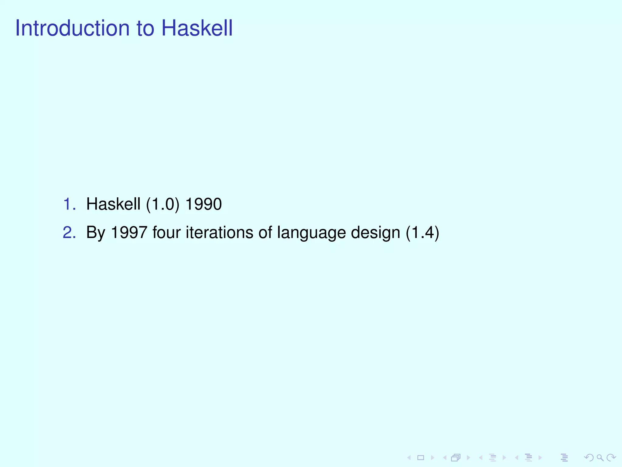

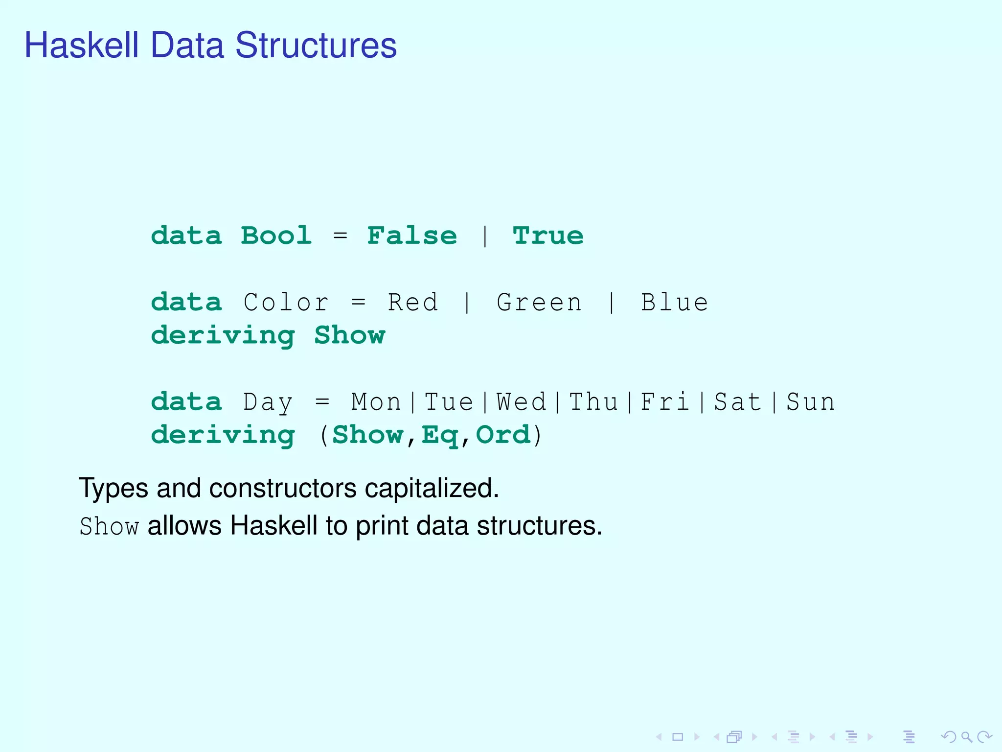
![Haskell
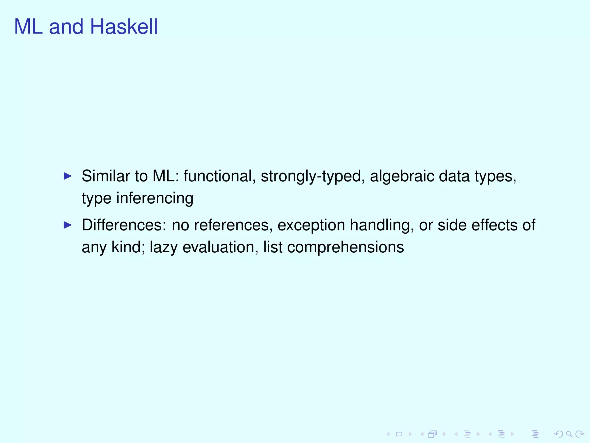
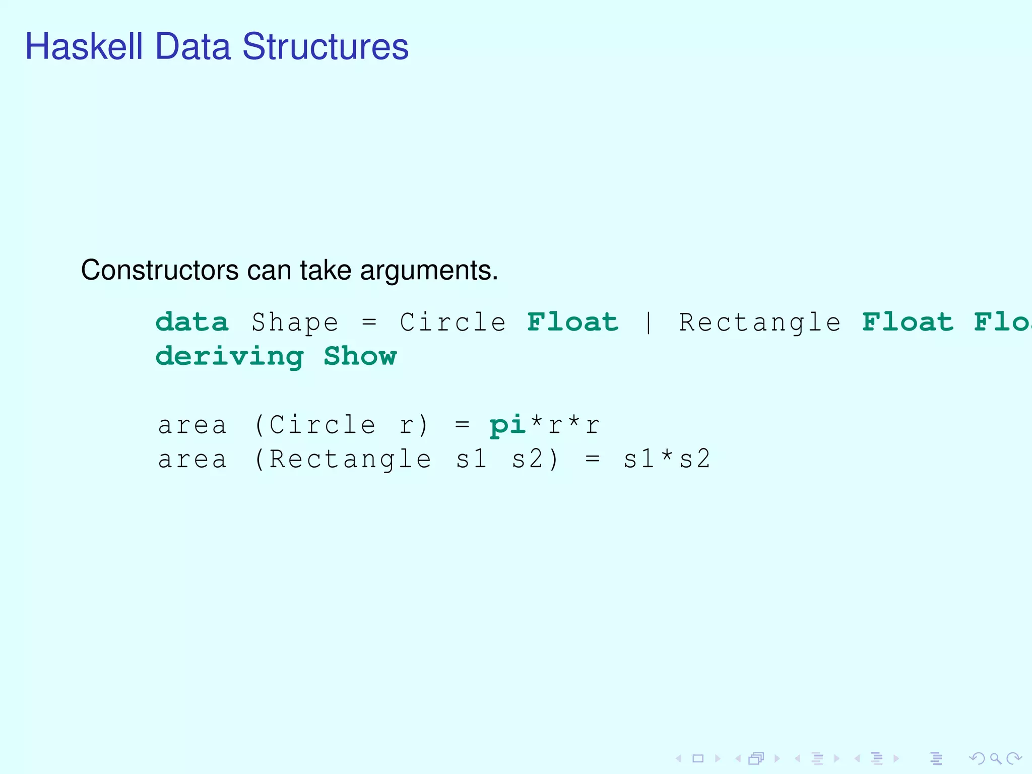
Similar to ML: functional, strongly-typed, algebraic data types,
type inferencing
Differences: no references, exception handling, or side effects of
any kind; lazy evaluation, list comprehensions
fac n = if n==0 then 1 else n * fac (n-1)
data Tree = Leaf | Node (Tree , String, Tree)
size (Leaf) = 1
size (Node (l,_,r)) = size (l) + size (r)
squares = [ n*n | n <- [0..] ]
pascal = iterate (row ->zipWith (+) ([0]++row) (row](https://image.slidesharecdn.com/fun-151224070521/75/Introduction-to-Functional-Languages-16-2048.jpg)
![Haskell List Comprehension
[e | x1 <- l1, ..., xm <- lm, P1, ..., Pn]
e is an expression, xi is a variable, li is a list, Pi is a predicate
[ xˆ2 | x <- [ 1..10 ], even x]
[ xˆ2 | x <- [ 2,4..10 ] ]
[ x+y | x <- [1..3], y <- [1..4] ]
perms [] = [[]]
perms x = [a:y | a<-x, y<-perms (x [a]) ]
quicksort [] = []
quicksort (s:xs) =
quicksort[x|x<-xs,x<s]++[s]++quicksort[x|x<-xs,x>=](https://image.slidesharecdn.com/fun-151224070521/75/Introduction-to-Functional-Languages-17-2048.jpg)
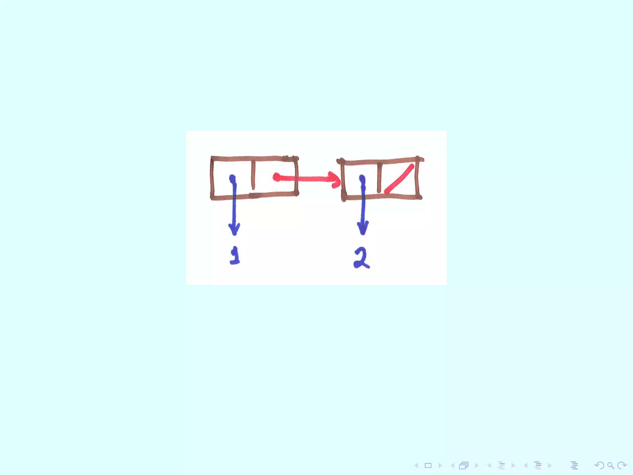
![Fold
foldr z[x1,x2,...,xn] = x1 (x2 (...(xn z)...))
foldr f z [x1, x2, ..., xn] = x1 f (x2 f (...(xn f z)...))](https://image.slidesharecdn.com/fun-151224070521/75/Introduction-to-Functional-Languages-26-2048.jpg)
![Fold
foldl z[x1,x2,...,xn] = (...((z x1) x2)...) xn
foldl f z [x1, x2, ..., xn] = (...((z f x1) f x2) ... ) f xn](https://image.slidesharecdn.com/fun-151224070521/75/Introduction-to-Functional-Languages-27-2048.jpg)
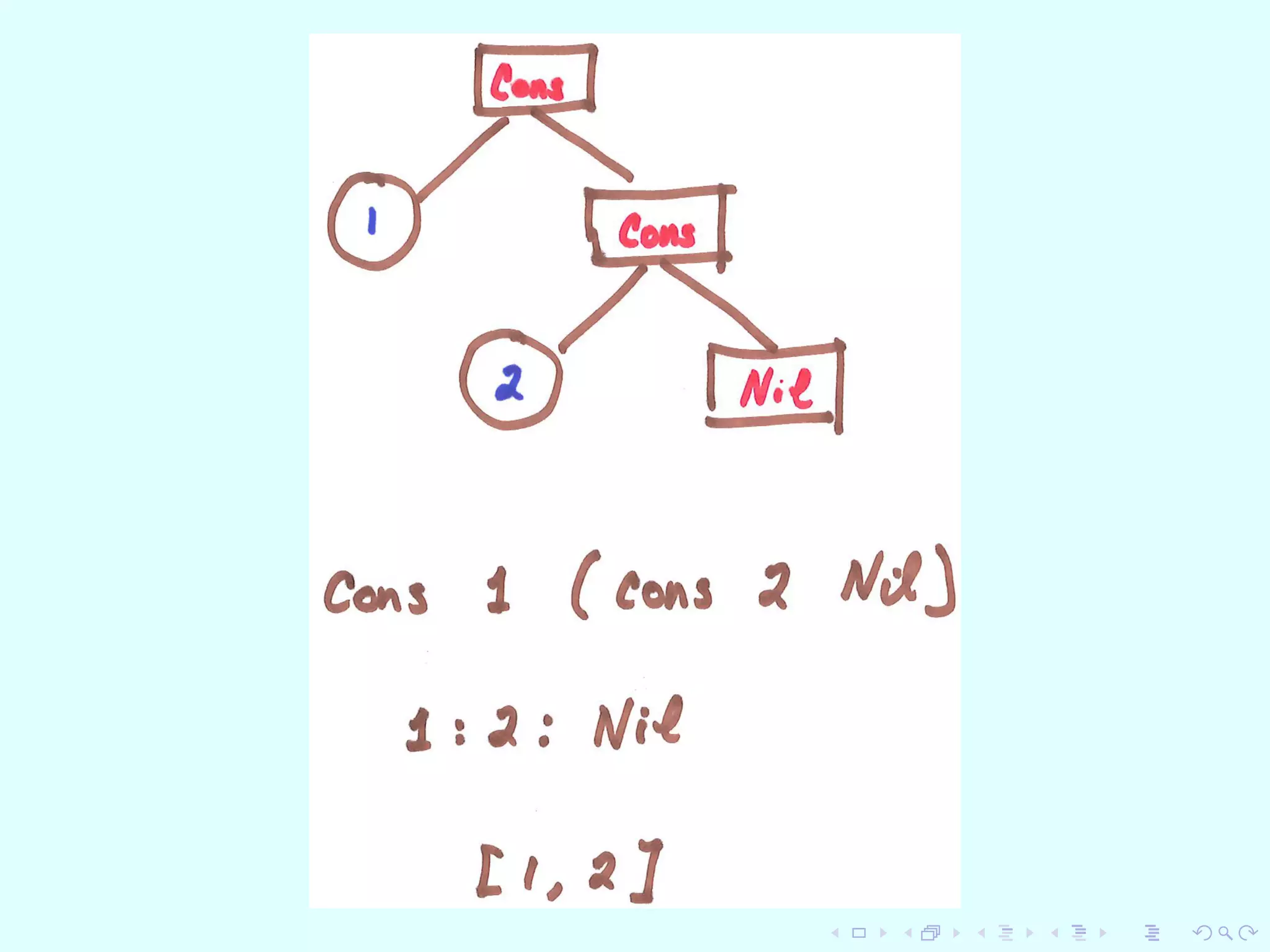
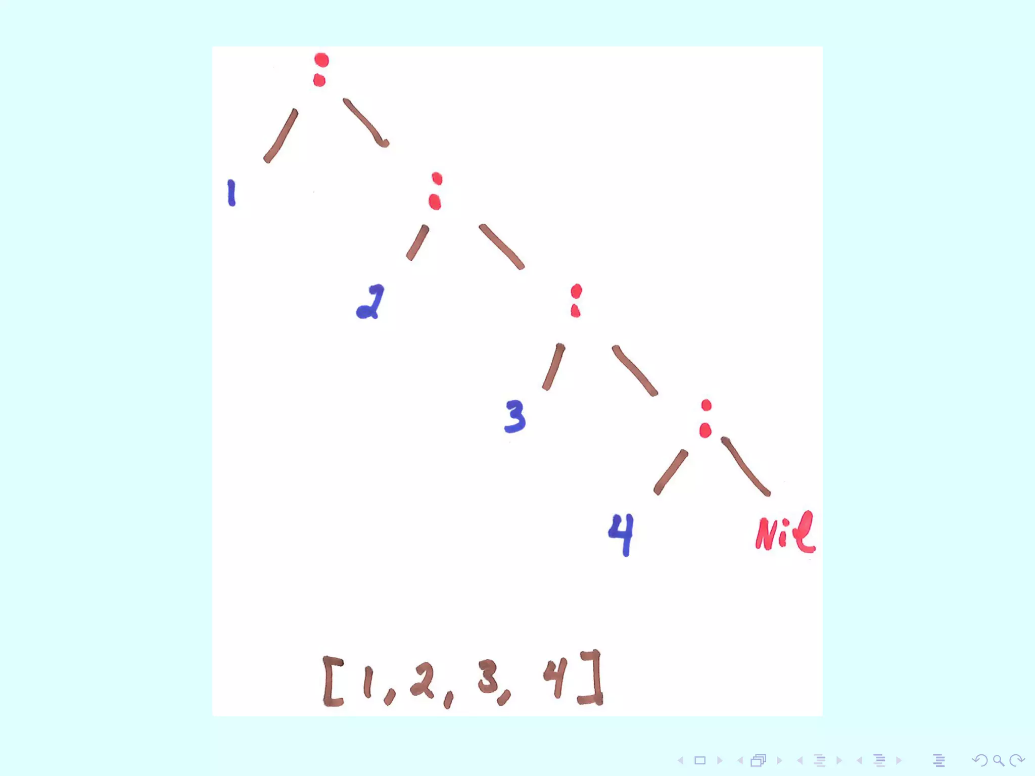
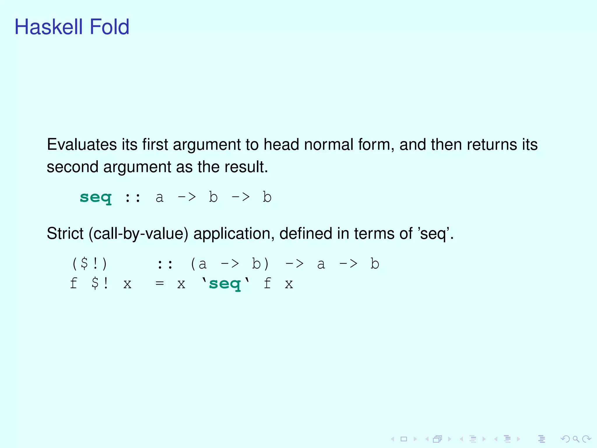
![Haskell Fold
foldr :: (b -> a -> a) -> a -> [b] ->
foldr f z [] = z
foldr f z (x:xs) = f x (foldr f z xs)
foldl :: (a -> b -> a) -> a -> [b] ->
foldl f z [] = z
foldl f z (x:xs) = foldl f (f z x) xs
foldl’ :: (a -> b -> a) -> a -> [b] -> a
foldl’ f z0 xs = foldr f’ id xs z0
where f’ x k z = k $! f z x
[Real World Haskell says never use foldl instead use foldl’.]](https://image.slidesharecdn.com/fun-151224070521/75/Introduction-to-Functional-Languages-28-2048.jpg)
![Haskell Fold
sum’ = foldl (+) 0
product’ = foldl (*) 1
and’ = foldl (&&) True
or’ = foldl (||) False
concat’ = foldl (++) []
composel = foldl (.) id
composer = foldr (.) id
length = foldl (const (+1)) 0
list_identity = foldr (:) []
reverse’ = foldl (flip (:)) []
unions = foldl Set.union Set.empty](https://image.slidesharecdn.com/fun-151224070521/75/Introduction-to-Functional-Languages-32-2048.jpg)
![Haskell Fold
reverse = foldl ( xs x -> xs ++ [x]) []
map f = foldl ( xs x -> f x : xs) []
filter p = foldl ( xs x -> if p x then x:xs el](https://image.slidesharecdn.com/fun-151224070521/75/Introduction-to-Functional-Languages-33-2048.jpg)
![Haskell Fold
If this is your pattern
g [] = v
g (x:xs) = f x (g xs)
then
g = foldr f v](https://image.slidesharecdn.com/fun-151224070521/75/Introduction-to-Functional-Languages-34-2048.jpg)
![Haskell Trees
See Hudak PPT, Ch7.
data SimpleTree = SimLeaf | SimBranch SimpleTree
data IntegerTree = IntLeaf Integer |
IntBranch IntegerTree IntegerTree
data InternalTree a = ILeaf |
IBranch a (InternalTree a) (InternalTree a)
data Tree a = Leaf a | Branch (Tree a) (Tree a)
data FancyTree a b = FLeaf a |
FBranch b (FancyTree a b) (FancyTree a b)
data GTree = GTree [GTree]
data GPTree a = GPTree a [GPTree a]](https://image.slidesharecdn.com/fun-151224070521/75/Introduction-to-Functional-Languages-41-2048.jpg)
![Haskell
input stream --> program --> output stream
Real World
[Char] --> program --> [Char]
Haskell World
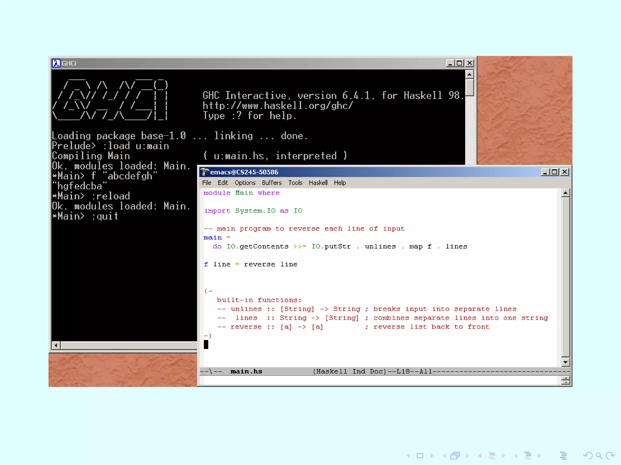
module Main where
main = do
input <- getContents
putStr $ unlines $ f $ lines input
countWords :: String -> String
countWords = unlines . format . count . words
count :: [String] -> [(String,Int)]
count = map (ws->(head ws, length ws))
. groupBy (==)
. sort](https://image.slidesharecdn.com/fun-151224070521/75/Introduction-to-Functional-Languages-43-2048.jpg)
![Haskell
input stream --> program --> output stream
Real World
[Char] --> program --> [Char]
Haskell World
module Main where
main = interact countWords
countWords :: String -> String
countWords = unlines . format . count . words
count :: [String] -> [(String,Int)]
count = map (ws->(head ws, length ws))
. groupBy (==)
. sort](https://image.slidesharecdn.com/fun-151224070521/75/Introduction-to-Functional-Languages-44-2048.jpg)

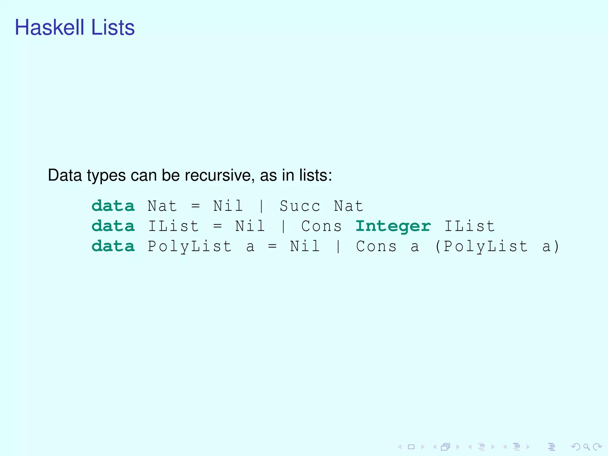
The document provides information about functional programming languages and concepts including: 1) Haskell and ML are introduced as functional languages with features like strong typing, algebraic data types, and pattern matching. 2) Core functional programming concepts are explained like referential transparency, higher-order functions, and recursion instead of iteration. 3) Fold functions are summarized as a way to iterate over lists in functional languages in both a left and right oriented way.


![[FLOLAC'14][scm] Functional Programming Using Haskell](https://cdn.slidesharecdn.com/ss_thumbnails/slides-140630030216-phpapp01-thumbnail.jpg?width=640&height=640&fit=bounds)