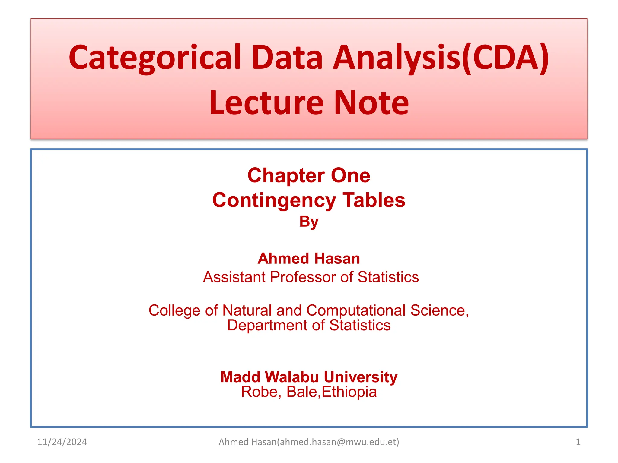
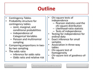
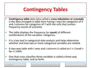
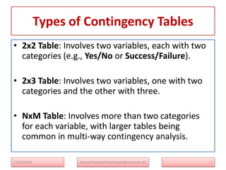
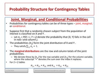
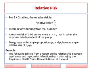
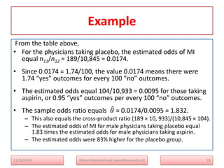
The document serves as a lecture note on categorical data analysis, focusing on contingency tables and their components, including probability structures, analysis methods, and measures of association. Key topics include chi-square tests for independence, relative risk, and odds ratios, along with their applications in comparing categorical data. The content emphasizes the importance of understanding relationships between categorical variables through various statistical approaches.

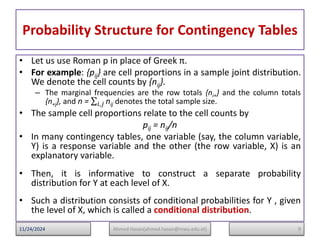
![Inference for Odds Ratios and Log
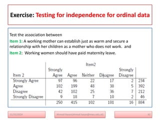
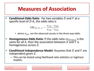
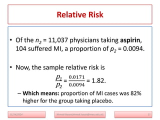
Odds Ratios
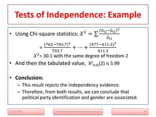
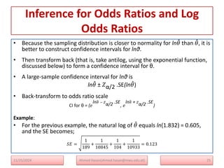
• For the population, a 95% confidence interval for lnθ equals
0.605 ± 1.96(0.123), or (0.365, 0.846).
• Back-transform to odds ratio scale: The corresponding confidence interval
for θ is
(e0.365, e0.846) = (1.44, 2.33)
• This is from the equality of ex = c is equivalent to ln(c) = x
– For instance, e0 = exp(0) = 1 corresponds to ln(1) = 0; similarly, e0.7 =
exp(0.7) = 2.0 corresponds to ln(2) = 0.7]
• Since the 95% confidence interval (1.44, 2.33) for the odds ratio does not
contain 1.0, the true odds of MI seem different for the two groups.
• We estimate that the odds of MI are at least 44% higher for subjects
taking placebo than for subjects taking aspirin.
26
Ahmed Hasan(ahmed.hasan@mwu.edu.et)
11/25/2024](https://image.slidesharecdn.com/ch-241208081723-f1370246/85/Introduction-to-Categorical-Data-Analysis-Contingency-Table-26-320.jpg)
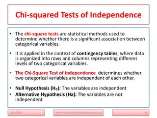
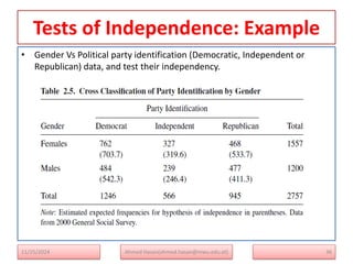
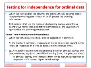
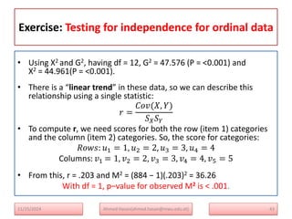
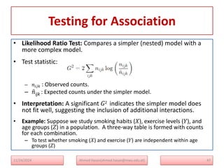
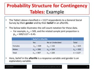
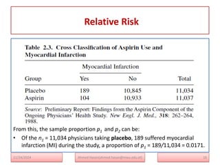
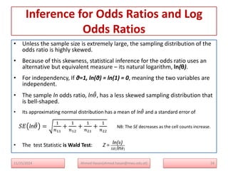
![Tests of Independence: Example
• Ho: political party identification and gender are Independent
Using likelihood test: G2 = 2 nij 𝒍𝒐𝒈
nij
µij
• The expected frequency, µij =
𝑛𝑖+𝑛+𝑗
𝑛
µ11 =
𝑛1+𝑛+1
𝑛
= µ11 =
1246∗1557
2757
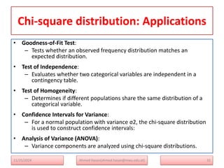
= 703.
µ12 =
𝑛1+𝑛+2
𝑛
= µ11 =
1557∗566
2757
= 319.6
……..
µ23 =
𝑛2+𝑛+3
𝑛
= µ23 =
1200∗945
2757
= 411.3
• Now, G2 = 2[762 log
762
703.7
+…+477 log
477
411.3
] = 30
• with (I-1)(J-1) =2 degree of freedom
37
Ahmed Hasan(ahmed.hasan@mwu.edu.et)
11/25/2024](https://image.slidesharecdn.com/ch-241208081723-f1370246/85/Introduction-to-Categorical-Data-Analysis-Contingency-Table-37-320.jpg)