This document describes implementing a modified particle filter algorithm for localization in an FPGA. The modified algorithm improves speed and accuracy. It was tested through simulations of global localization, localization and tracking, and kidnapping scenarios. The hardware implementation was 34x faster than software and successfully localized the robot in all experiments, demonstrating the FPGA is capable of running the particle filter in real-time.

1. Implement a modified algorithm
PF in a FPGA
27/11/2015
Bruno Martínez
馬博彥
CIR Lab

2. Outline
• Implement a modified algorithm PF in a FPGA
– Modified algorithm PF
– Designed blocks
– Designed VHDL code
– State Machine
– Analyze and Synthesize
– Program FPGA
p.1

3. Particle filter algorithm
1. Initialization
Create randomly 500 particles and jump to step 4
2. Prediction of the particles pose
If the robot is moving, the best 5 particles move 8 pixels
3. Distribution of the particles
Distribute particles around the best 5 particles
4. Calculation of the particle weight
Compared lasers from the real robot with lasers of each particle
as a determination of weight (importance factor)
5. Choice of the best 5 particles
Choosing the best 5 particles with the lowest weight, and jump
to step 2
p.2

4. Features and improvements
Resolution of the Map:
• 594x804 pixels
• 1 pixel = 8 cm
Lasers of the Robot:
• Maximum distance 800 cm
• 37 lasers with 5º each
Movements of the Robot:
• Moves straightforward: 8 pixels = 64 cm
• Turns 10º either right or left
p.3

5. Features and improvements
Proposed PF:
• Rank of distribution for the new particles
(15,15)
• Particles with lower weight < 100:
• 200 particles instead of 500
• Rank of distribution (3,3)
• Particles with lower weight > 250 and
number of iterations > 50:
• Distribute 500 particles all over the
map
p.4

6. Features
• Improvement of the hardware design speed:
All particles are saved in 5 RAMs, each RAM contains 100 particles.
If PF is using 500 particles or 40 particles, if PF is using 200
particles. Then it can operate simultaneously and faster.
p.5

7. Blocks - Diagram
p.6

8. Memory - Diagrams
p.7

9. State Machine
S2: Initialization
S3: Particle Update
S4: Distribution
S5: Calculate Weight
S6: Select 5 Best Weights
p.8

10. Verification of hardware design
Simulations of pose tracking on ModelSim, where the robot position
is noticed as (PosXRo, PosYRo, AngRo) and the estimated pose of
the proposed PF is denoted as (oPosXBP, oPosYBP, o AngBP).
p.9

11. Implementation in FPGA
Flow Summary
Total logic elements 30,651 / 149,760 ( 20 % )
Total registers 6,752
Total pins 90 / 508 ( 18 % )
Total memory bits 32,752 / 6,635,520 ( < 1 % )
Embedded Multiplier 9-bit elements 20 / 720 ( 3 % )
Development Kit: DE2i-150 FPGA
FPGA: Cyclone IV GX
p.10

12. Results
3 different experiments:
• Global localization
• Global localization and pose tracking
• Kidnapping
p.11

13. Noise
• Lasers:
There are several experiments employing different noise values,
but the results shown here is ±5 pixels random noise for each laser.
This is a very intense noise.
• Odometer:
The robot moves 8 pixels, and a ±2 pixels random error is introduced.
p.12

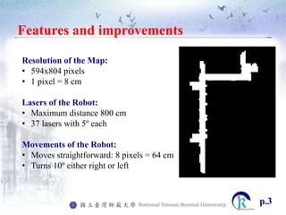
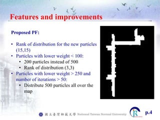
14. Global Localization
SW HW
Weight of the particle which
estimates the pose of the robot
105 94
Difference between true and
estimated pose
[0.4, 1] [0, 0.8]
Time to localize the robot 2.655 s 0.119 s
Number of iterations of the
algorithm
14 24
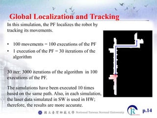
The results come from an experiment with the function of localizing the
robot in a specific location.
The simulations have been executed 10 times, and the below table
demonstrates the average of these 10 attempts.
p.13

15. Global Localization and Tracking
In this simulation, the PF localizes the robot by
tracking its movements.
• 100 movements = 100 executions of the PF
• 1 execution of the PF = 30 iterations of the
algorithm
30 iter: 3000 iterations of the algorithm in 100
executions of the PF.
The simulations have been executed 10 times
based on the same path. Also, in each simulation,
the laser data simulated in SW is used in HW;
therefore, the results are more accurate.
p.14

16. Global Localization and Tracking
Δx (px) Δy (px) Δo (º) √(Δx)^2+(Δy)^2 (px) Time (s)
SW 0.394 0.258 0.000 0.474 210.60
HW 0.480 0.450 0.000 0.660 6.23
In the table below, the error is a little bit bigger in HW because it is less
accurate due to sine and cosine functions. However, considering the
computational time, HW outperforms SW.
p.15

17. Kidnapping
The PF localizes the robot correctly, but after 5 movements, the robot is
moved to another localization, then the PF has to localize again, as fast
as possible.
p.16

18. Kidnapping
The PF re-localizes the robot in one execution, less than 30 iterations.
Therefore the PF never loses the robot.
The experiment has been executed 10 times, the below table
demonstrates the average of these 10 attempts:
Δx (px) Δy (px) Δo (º) √(Δx)^2+(Δy)^2 (px)
SW 0.300 0.300 0.000 0.424
HW 0.200 0.500 0.000 0.539
p.17

19. Conclusions
• Robust localization method
• HW platform 34x faster than SW
• Enough resources to implement the method in the FPGA
p.18