Weeks 1 &2 2
Introduction to the course
Introduction to the course
► Textbooks:
f
► Slides: available
►Lab: using Matlab
3.
Weeks 1 &2 3
Introduction to the course
Introduction to the course
► Grading
Attendance: 10%
Assignments: 10%
Midterm: 20%
Project: 20%
Final: 40%
Total: 100%
4.
Weeks 1 &2 4
Introduction to the course
Introduction to the course
► Project
Medical image analysis (MRI/PET/CT/X-ray tumor
detection/classification)
Face, fingerprint, and other object recognition
Image and/or video compression
Image segmentation and/or denoising
Digital image/video watermarking/steganography
and detection
5.
Weeks 1 &2 5
Introduction to the course
Introduction to the course
► Evaluation of project
Report
Project
— Submit an article including introduction, methods,
experiments, results, and conclusions
— Submit the project code, the readme document, and some
testing samples (images, videos, etc.) for validation
Presentation
6.
Weeks 1 &2 6
Journals & Conferences
Journals & Conferences
in Image Processing
in Image Processing
► Journals:
— IEEE T IMAGE PROCESSING
— IEEE T MEDICAL IMAGING
— INTL J COMP. VISION
— IEEE T PATTERN ANALYSIS MACHINE INTELLIGENCE
— PATTERN RECOGNITION
— COMP. VISION AND IMAGE UNDERSTANDING
— IMAGE AND VISION COMPUTING
… …
► Conferences:
— CVPR: Comp. Vision and Pattern Recognition
— ICCV: Intl Conf on Computer Vision
— ACM Multimedia
— ICIP
— SPIE
— ECCV: European Conf on Computer Vision
— CAIP: Intl Conf on Comp. Analysis of Images and Patterns
… …
7.
Weeks 1 &2 7
Introduction
Introduction
► What is Digital Image Processing?
Digital Image
— a two-dimensional function
x and y are spatial coordinates
The amplitude of f is called intensity or gray level at the point (x, y)
Digital Image Processing
— process digital images by means of computer, it covers low-, mid-, and high-level
processes
low-level: inputs and outputs are images
mid-level: outputs are attributes extracted from input images
high-level: an ensemble of recognition of individual objects
Pixel
— the elements of a digital image
( , )
f x y
8.
Weeks 1 &2 8
Origins of Digital Image
Origins of Digital Image
Processing
Processing
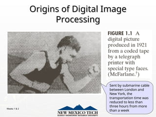
Sent by submarine cable
between London and
New York, the
transportation time was
reduced to less than
three hours from more
than a week
9.
Weeks 1 &2 9
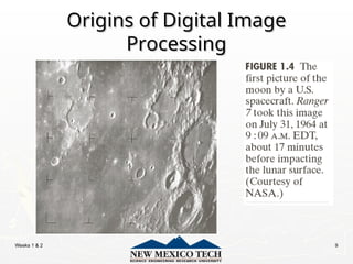
Origins of Digital Image
Origins of Digital Image
Processing
Processing
10.
Weeks 1 &2 10
Sources for Images
Sources for Images
► Electromagnetic (EM) energy spectrum
Electromagnetic (EM) energy spectrum
► Acoustic
Acoustic
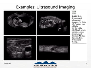
► Ultrasonic
Ultrasonic
► Electronic
Electronic
► Synthetic images produced by computer
Synthetic images produced by computer
11.
Weeks 1 &2 11
Electromagnetic (EM) energy spectrum
Electromagnetic (EM) energy spectrum
Major uses
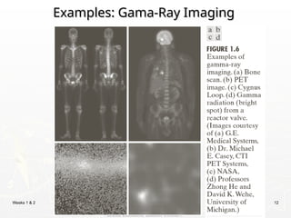
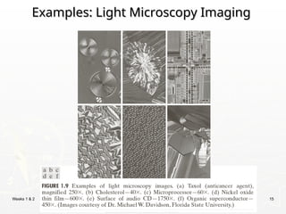
Gamma-ray imaging: nuclear medicine and astronomical observations
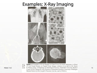
X-rays: medical diagnostics, industry, and astronomy, etc.
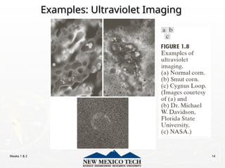
Ultraviolet: lithography, industrial inspection, microscopy, lasers, biological imaging,
and astronomical observations
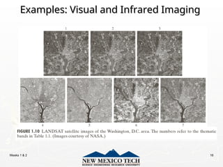
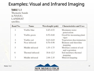
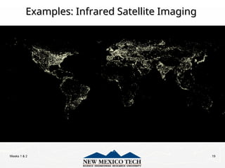
Visible and infrared bands: light microscopy, astronomy, remote sensing, industry,
and law enforcement
Microwave band: radar
Radio band: medicine (such as MRI) and astronomy
Weeks 1 &2 21
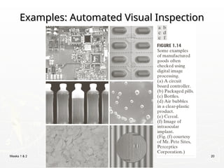
Examples: Automated Visual Inspection
Examples: Automated Visual Inspection
The area in
which the
imaging system
detected the
plate
Results of
automated
reading of the
plate content
by the system
22.
Weeks 1 &2 22
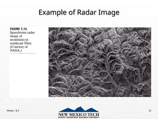
Example of Radar Image
Example of Radar Image
Weeks 1 &2 25
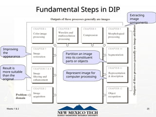
Fundamental Steps in DIP
Fundamental Steps in DIP
Result is
more suitable
than the
original
Improving
the
appearance
Extracting
image
components
Partition an image
into its constituent
parts or objects
Represent image for
computer processing
26.
Weeks 1 &2 26
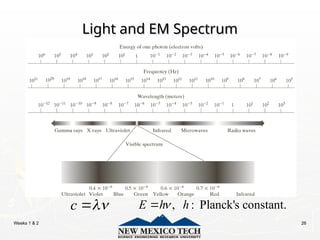
Light and EM Spectrum
Light and EM Spectrum
c
, : Planck's constant.
E h h
27.
Weeks 1 &2 27
Light and EM Spectrum
Light and EM Spectrum
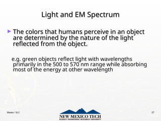
► The colors that humans perceive in an object
The colors that humans perceive in an object
are determined by the nature of the light
are determined by the nature of the light
reflected from the object.
reflected from the object.
e.g. green objects reflect light with wavelengths
primarily in the 500 to 570 nm range while absorbing
most of the energy at other wavelength
28.
Weeks 1 &2 28
Light and EM Spectrum
Light and EM Spectrum
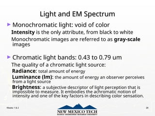
► Monochromatic light: void of color
Intensity is the only attribute, from black to white
Monochromatic images are referred to as gray-scale
images
► Chromatic light bands: 0.43 to 0.79 um
The quality of a chromatic light source:
Radiance: total amount of energy
Luminance (lm): the amount of energy an observer perceives
from a light source
Brightness: a subjective descriptor of light perception that is
impossible to measure. It embodies the achromatic notion of
intensity and one of the key factors in describing color sensation.
29.
Weeks 1 &2 29
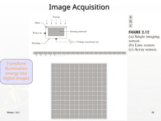
Image Acquisition
Image Acquisition
Transform
illumination
energy into
digital images
30.
Weeks 1 &2 30
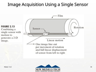
Image Acquisition Using a Single Sensor
Image Acquisition Using a Single Sensor
31.
Weeks 1 &2 31
Image Acquisition Using Sensor Strips
Image Acquisition Using Sensor Strips
32.
Weeks 1 &2 32
Image Acquisition Process
Image Acquisition Process
33.
Weeks 1 &2 33
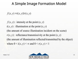
A Simple Image Formation Model
A Simple Image Formation Model
( , ) ( , ) ( , )
( , ): intensity at the point ( , )
( , ): illumination at the point ( , )
(the amount of source illumination incident on the scene)
( , ): reflectance/transmissivity
f x y i x y r x y
f x y x y
i x y x y
r x y
at the point ( , )
(the amount of illumination reflected/transmitted by the object)
where 0 < ( , ) < and 0 < ( , ) < 1
x y
i x y r x y
34.
Weeks 1 &2 34
Some Typical Ranges of illumination
Some Typical Ranges of illumination
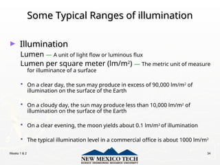
► Illumination
Illumination
Lumen — A unit of light flow or luminous flux
Lumen per square meter (lm/m2
) — The metric unit of measure
for illuminance of a surface
On a clear day, the sun may produce in excess of 90,000 lm/m2
of
illumination on the surface of the Earth
On a cloudy day, the sun may produce less than 10,000 lm/m2
of
illumination on the surface of the Earth
On a clear evening, the moon yields about 0.1 lm/m2
of illumination
The typical illumination level in a commercial office is about 1000 lm/m2
35.
Weeks 1 &2 35
Some Typical Ranges of Reflectance
Some Typical Ranges of Reflectance
► Reflectance
Reflectance
0.01 for black velvet
0.65 for stainless steel
0.80 for flat-white wall paint
0.90 for silver-plated metal
0.93 for snow
36.
Weeks 1 &2 36
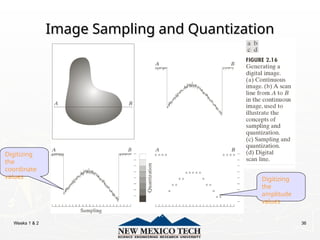
Image Sampling and Quantization
Image Sampling and Quantization
Digitizing
the
coordinate
values Digitizing
the
amplitude
values
37.
Weeks 1 &2 37
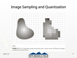
Image Sampling and Quantization
Image Sampling and Quantization
38.
Weeks 1 &2 38
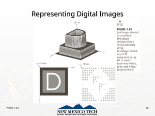
Representing Digital Images
Representing Digital Images
39.
Weeks 1 &2 39
Representing Digital Images
Representing Digital Images
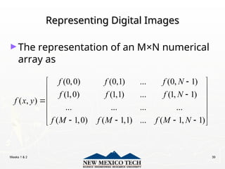
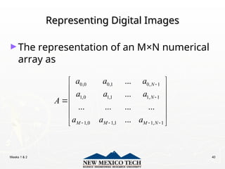
►The representation of an M×N numerical
array as
(0,0) (0,1) ... (0, 1)
(1,0) (1,1) ... (1, 1)
( , )
... ... ... ...
( 1,0) ( 1,1) ... ( 1, 1)
f f f N
f f f N
f x y
f M f M f M N
40.
Weeks 1 &2 40
Representing Digital Images
Representing Digital Images
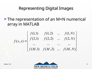
►The representation of an M×N numerical
array as
0,0 0,1 0, 1
1,0 1,1 1, 1
1,0 1,1 1, 1
...
...
... ... ... ...
...
N
N
M M M N
a a a
a a a
A
a a a
41.
Weeks 1 &2 41
Representing Digital Images
Representing Digital Images
►The representation of an M×N numerical
array in MATLAB
(1,1) (1,2) ... (1, )
(2,1) (2,2) ... (2, )
( , )
... ... ... ...
( ,1) ( ,2) ... ( , )
f f f N
f f f N
f x y
f M f M f M N
42.
Weeks 1 &2 42
Representing Digital Images
Representing Digital Images
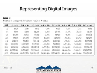
► Discrete intensity interval [0, L-1], L=2k
► The number b of bits required to store a M × N
digitized image
b = M × N × k
43.
Weeks 1 &2 43
Representing Digital Images
Representing Digital Images
44.
Weeks 1 &2 44
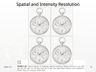
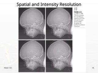
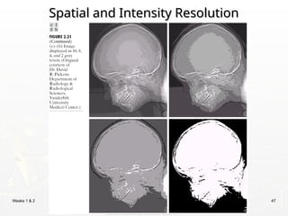
Spatial and Intensity Resolution
Spatial and Intensity Resolution
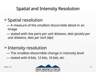
►Spatial resolution
— A measure of the smallest discernible detail in an
image
— stated with line pairs per unit distance, dots (pixels) per
unit distance, dots per inch (dpi)
►Intensity resolution
— The smallest discernible change in intensity level
— stated with 8 bits, 12 bits, 16 bits, etc.
45.
Weeks 1 &2 45
Spatial and Intensity Resolution
Spatial and Intensity Resolution
46.
Weeks 1 &2 46
Spatial and Intensity Resolution
Spatial and Intensity Resolution
47.
Weeks 1 &2 47
Spatial and Intensity Resolution
Spatial and Intensity Resolution
48.
Weeks 1 &2 48
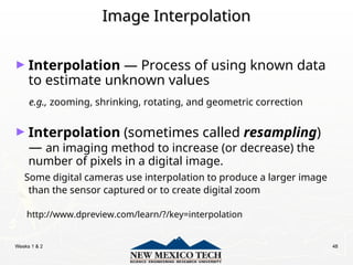
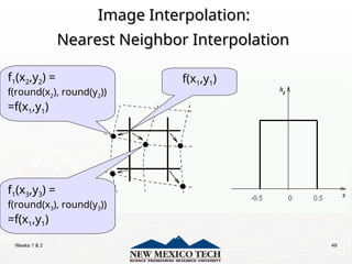
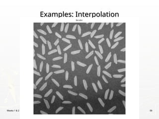
Image Interpolation
Image Interpolation
► Interpolation — Process of using known data
to estimate unknown values
e.g., zooming, shrinking, rotating, and geometric correction
► Interpolation (sometimes called resampling)
— an imaging method to increase (or decrease) the
number of pixels in a digital image.
Some digital cameras use interpolation to produce a larger image
than the sensor captured or to create digital zoom
http://www.dpreview.com/learn/?/key=interpolation
Weeks 1 &2 50
Image Interpolation:
Image Interpolation:
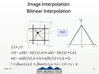
Bilinear Interpolation
Bilinear Interpolation
2 ( , )
(1 ) (1 ) ( , ) (1 ) ( 1, )
(1 ) ( , 1) ( 1, 1)
( ), ( ), , .
f x y
a b f l k a b f l k
a b f l k a b f l k
l floor x k floor y a x l b y k
(x,y)
51.
Weeks 1 &2 51
Image Interpolation:
Image Interpolation:
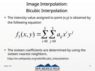
Bicubic Interpolation
Bicubic Interpolation
3 3
3
0 0
( , ) i j
ij
i j
f x y a x y
► The intensity value assigned to point (x,y) is obtained by
the following equation
► The sixteen coefficients are determined by using the
sixteen nearest neighbors.
http://en.wikipedia.org/wiki/Bicubic_interpolation
Weeks 1 &2 60
Basic Relationships Between Pixels
► Neighborhood
► Adjacency
► Connectivity
► Paths
► Regions and boundaries
61.
Weeks 1 &2 61
Basic Relationships Between Pixels
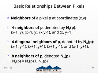
► Neighbors of a pixel p at coordinates (x,y)
4-neighbors of p, denoted by N4(p):
(x-1, y), (x+1, y), (x,y-1), and (x, y+1).
4 diagonal neighbors of p, denoted by ND(p):
(x-1, y-1), (x+1, y+1), (x+1,y-1), and (x-1, y+1).
8 neighbors of p, denoted N8(p)
N8(p) = N4(p) U ND(p)
62.
Weeks 1 &2 62
Basic Relationships Between Pixels
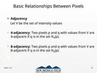
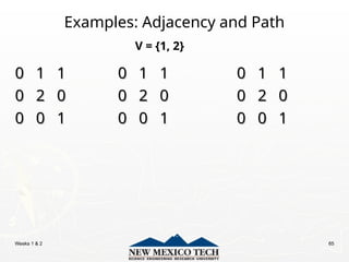
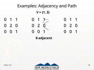
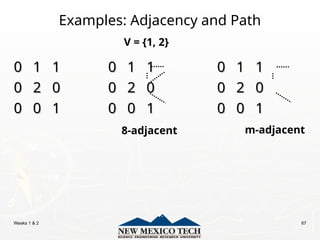
► Adjacency
Let V be the set of intensity values
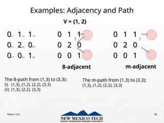
4-adjacency: Two pixels p and q with values from V are
4-adjacent if q is in the set N4(p).
8-adjacency: Two pixels p and q with values from V are
8-adjacent if q is in the set N8(p).
63.
Weeks 1 &2 63
Basic Relationships Between Pixels
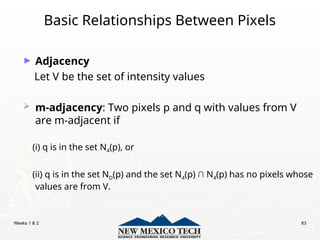
► Adjacency
Let V be the set of intensity values
m-adjacency: Two pixels p and q with values from V
are m-adjacent if
(i) q is in the set N4(p), or
(ii) q is in the set ND(p) and the set N4(p) ∩ N4(p) has no pixels whose
values are from V.
64.
Weeks 1 &2 64
Basic Relationships Between Pixels
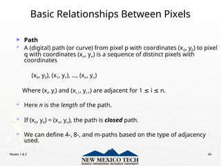
► Path
A (digital) path (or curve) from pixel p with coordinates (x0, y0) to pixel
q with coordinates (xn, yn) is a sequence of distinct pixels with
coordinates
(x0, y0), (x1, y1), …, (xn, yn)
Where (xi, yi) and (xi-1, yi-1) are adjacent for 1 i n.
≤ ≤
Here n is the length of the path.
If (x0, y0) = (xn, yn), the path is closed path.
We can define 4-, 8-, and m-paths based on the type of adjacency
used.
Weeks 1 &2 69
Basic Relationships Between Pixels
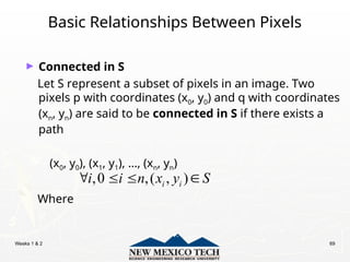
► Connected in S
Let S represent a subset of pixels in an image. Two
pixels p with coordinates (x0, y0) and q with coordinates
(xn, yn) are said to be connected in S if there exists a
path
(x0, y0), (x1, y1), …, (xn, yn)
Where
,0 ,( , )
i i
i i n x y S
70.
Weeks 1 &2 70
Basic Relationships Between Pixels
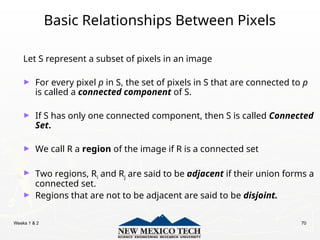
Let S represent a subset of pixels in an image
► For every pixel p in S, the set of pixels in S that are connected to p
is called a connected component of S.
► If S has only one connected component, then S is called Connected
Set.
► We call R a region of the image if R is a connected set
► Two regions, Ri and Rj are said to be adjacent if their union forms a
connected set.
► Regions that are not to be adjacent are said to be disjoint.
71.
Weeks 1 &2 71
Basic Relationships Between Pixels
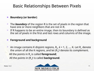
► Boundary (or border)
The boundary of the region R is the set of pixels in the region that
have one or more neighbors that are not in R.
If R happens to be an entire image, then its boundary is defined as
the set of pixels in the first and last rows and columns of the image.
► Foreground and background
An image contains K disjoint regions, Rk, k = 1, 2, …, K. Let Ru denote
the union of all the K regions, and let (Ru)c
denote its complement.
All the points in Ru is called foreground;
All the points in (Ru)c
is called background.
72.
Weeks 1 &2 72
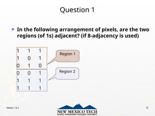
Question 1
► In the following arrangement of pixels, are the two
regions (of 1s) adjacent? (if 8-adjacency is used)
1 1 1
1 0 1
0 1 0
0 0 1
1 1 1
1 1 1
Region 1
Region 2
73.
Weeks 1 &2 73
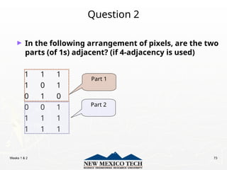
Question 2
► In the following arrangement of pixels, are the two
parts (of 1s) adjacent? (if 4-adjacency is used)
1 1 1
1 0 1
0 1 0
0 0 1
1 1 1
1 1 1
Part 1
Part 2
74.
Weeks 1 &2 74
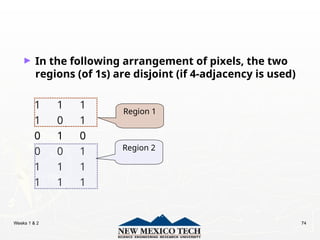
► In the following arrangement of pixels, the two
regions (of 1s) are disjoint (if 4-adjacency is used)
1 1 1
1 0 1
0 1 0
0 0 1
1 1 1
1 1 1
Region 1
Region 2
75.
Weeks 1 &2 75
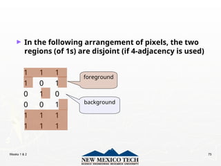
► In the following arrangement of pixels, the two
regions (of 1s) are disjoint (if 4-adjacency is used)
1 1 1
1 0 1
0 1 0
0 0 1
1 1 1
1 1 1
foreground
background
76.
Weeks 1 &2 76
Question 3
► In the following arrangement of pixels, the circled
point is part of the boundary of the 1-valued pixels if
8-adjacency is used, true or false?
0 0 0 0 0
0 1 1 0 0
0 1 1 0 0
0 1 1 1 0
0 1 1 1 0
0 0 0 0 0
77.
Weeks 1 &2 77
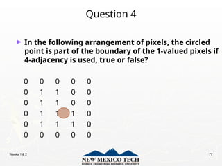
Question 4
► In the following arrangement of pixels, the circled
point is part of the boundary of the 1-valued pixels if
4-adjacency is used, true or false?
0 0 0 0 0
0 1 1 0 0
0 1 1 0 0
0 1 1 1 0
0 1 1 1 0
0 0 0 0 0
78.
Weeks 1 &2 78
Distance Measures
► Given pixels p, q and z with coordinates (x, y), (s, t),
(u, v) respectively, the distance function D has
following properties:
a. D(p, q) ≥ 0 [D(p, q) = 0, iff p = q]
b. D(p, q) = D(q, p)
c. D(p, z) ≤ D(p, q) + D(q, z)
79.
Weeks 1 &2 79
Distance Measures
The following are the different Distance measures:
a. Euclidean Distance :
De(p, q) = [(x-s)2
+ (y-t)2
]1/2
b. City Block Distance:
D4(p, q) = |x-s| + |y-t|
c. Chess Board Distance:
D8(p, q) = max(|x-s|, |y-t|)
80.
Weeks 1 &2 80
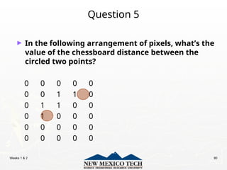
Question 5
► In the following arrangement of pixels, what’s the
value of the chessboard distance between the
circled two points?
0 0 0 0 0
0 0 1 1 0
0 1 1 0 0
0 1 0 0 0
0 0 0 0 0
0 0 0 0 0
81.
Weeks 1 &2 81
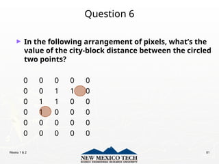
Question 6
► In the following arrangement of pixels, what’s the
value of the city-block distance between the circled
two points?
0 0 0 0 0
0 0 1 1 0
0 1 1 0 0
0 1 0 0 0
0 0 0 0 0
0 0 0 0 0
82.
Weeks 1 &2 82
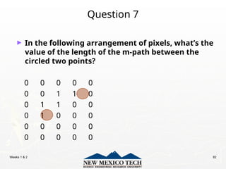
Question 7
► In the following arrangement of pixels, what’s the
value of the length of the m-path between the
circled two points?
0 0 0 0 0
0 0 1 1 0
0 1 1 0 0
0 1 0 0 0
0 0 0 0 0
0 0 0 0 0
83.
Weeks 1 &2 83
Question 8
► In the following arrangement of pixels, what’s the
value of the length of the m-path between the
circled two points?
0 0 0 0 0
0 0 1 1 0
0 0 1 0 0
0 1 0 0 0
0 0 0 0 0
0 0 0 0 0
84.
Weeks 1 &2 84
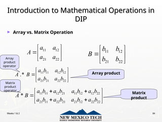
Introduction to Mathematical Operations in
Introduction to Mathematical Operations in
DIP
DIP
► Array vs. Matrix Operation
11 12
21 22
b b
B
b b
11 12
21 22
a a
A
a a
11 11 12 21 11 12 12 22
21 11 22 21 21 12 22 22
*
a b a b a b a b
A B
a b a b a b a b
11 11 12 12
21 21 22 22
.*
a b a b
A B
a b a b
Array product
Matrix
product
Array
product
operator
Matrix
product
operator
85.
Weeks 1 &2 85
Introduction to Mathematical Operations in
Introduction to Mathematical Operations in
DIP
DIP
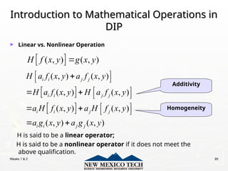
► Linear vs. Nonlinear Operation
H is said to be a linear operator;
H is said to be a nonlinear operator if it does not meet the
above qualification.
( , ) ( , )
H f x y g x y
Additivity
Homogeneity
( , ) ( , )
( , ) ( , )
( , ) ( , )
( , ) ( , )
i i j j
i i j j
i i j j
i i j j
H a f x y a f x y
H a f x y H a f x y
a H f x y a H f x y
a g x y a g x y
86.
Weeks 1 &2 86
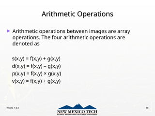
Arithmetic Operations
Arithmetic Operations
► Arithmetic operations between images are array
operations. The four arithmetic operations are
denoted as
s(x,y) = f(x,y) + g(x,y)
d(x,y) = f(x,y) – g(x,y)
p(x,y) = f(x,y) × g(x,y)
v(x,y) = f(x,y) ÷ g(x,y)
87.
Weeks 1 &2 87
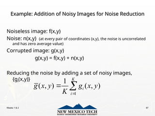
Example: Addition of Noisy Images for Noise Reduction
Example: Addition of Noisy Images for Noise Reduction
Noiseless image: f(x,y)
Noise: n(x,y) (at every pair of coordinates (x,y), the noise is uncorrelated
and has zero average value)
Corrupted image: g(x,y)
g(x,y) = f(x,y) + n(x,y)
Reducing the noise by adding a set of noisy images,
{gi(x,y)}
1
1
( , ) ( , )
K
i
i
g x y g x y
K
88.
Weeks 1 &2 88
Example: Addition of Noisy Images for Noise Reduction
Example: Addition of Noisy Images for Noise Reduction
1
1
1
1
( , ) ( , )
1
( , ) ( , )
1
( , ) ( , )
( , )
K
i
i
K
i
i
K
i
i
E g x y E g x y
K
E f x y n x y
K
f x y E n x y
K
f x y
1
1
( , ) ( , )
K
i
i
g x y g x y
K
2
( , ) 1
( , )
1
1
( , )
1
2
2 2
( , )
1
g x y K
g x y
i
K i
K
n x y
i
K i
n x y
K
89.
Weeks 1 &2 89
Example: Addition of Noisy Images for Noise Reduction
Example: Addition of Noisy Images for Noise Reduction
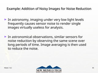
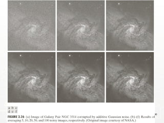
► In astronomy, imaging under very low light levels
frequently causes sensor noise to render single
images virtually useless for analysis.
► In astronomical observations, similar sensors for
noise reduction by observing the same scene over
long periods of time. Image averaging is then used
to reduce the noise.
Weeks 1 &2 91
An Example of Image Subtraction: Mask Mode
An Example of Image Subtraction: Mask Mode
Radiography
Radiography
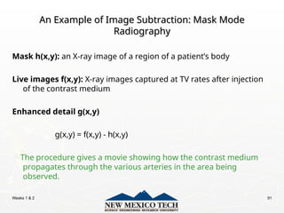
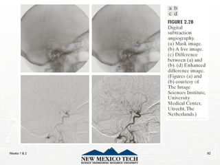
Mask h(x,y): an X-ray image of a region of a patient’s body
Live images f(x,y): X-ray images captured at TV rates after injection
of the contrast medium
Enhanced detail g(x,y)
g(x,y) = f(x,y) - h(x,y)
The procedure gives a movie showing how the contrast medium
propagates through the various arteries in the area being
observed.
Weeks 1 &2 93
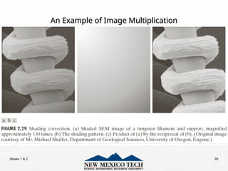
An Example of Image Multiplication
An Example of Image Multiplication
94.
Weeks 1 &2 94
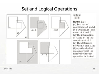
Set and Logical Operations
Set and Logical Operations
95.
Weeks 1 &2 95
Set and Logical Operations
Set and Logical Operations
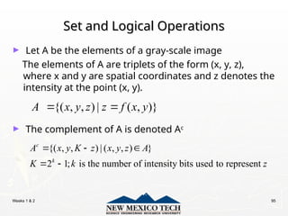
► Let A be the elements of a gray-scale image
The elements of A are triplets of the form (x, y, z),
where x and y are spatial coordinates and z denotes the
intensity at the point (x, y).
► The complement of A is denoted Ac
{( , , ) | ( , , ) }
2 1; is the number of intensity bits used to represent
c
k
A x y K z x y z A
K k z
{( , , ) | ( , )}
A x y z z f x y
96.
Weeks 1 &2 96
Set and Logical Operations
Set and Logical Operations
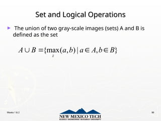
► The union of two gray-scale images (sets) A and B is
defined as the set
{max( , ) | , }
z
A B a b a A b B
97.
Weeks 1 &2 97
Set and Logical Operations
Set and Logical Operations
98.
Weeks 1 &2 98
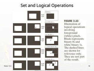
Set and Logical Operations
Set and Logical Operations
99.
Weeks 1 &2 99
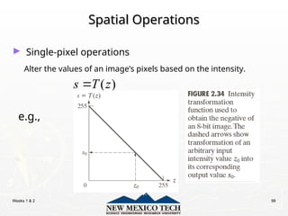
Spatial Operations
Spatial Operations
► Single-pixel operations
Alter the values of an image’s pixels based on the intensity.
e.g.,
( )
s T z
100.
Weeks 1 &2 100
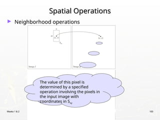
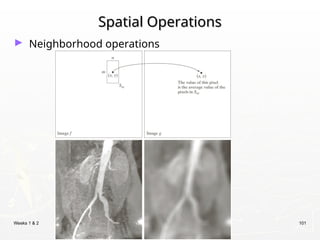
Spatial Operations
Spatial Operations
► Neighborhood operations
The value of this pixel is
determined by a specified
operation involving the pixels in
the input image with
coordinates in Sxy
Weeks 1 &2 102
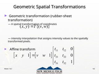
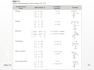
Geometric Spatial Transformations
Geometric Spatial Transformations
► Geometric transformation (rubber-sheet
transformation)
— A spatial transformation of coordinates
— intensity interpolation that assigns intensity values to the spatially
transformed pixels.
► Affine transform
( , ) {( , )}
x y T v w
11 12
21 22
31 32
0
1 1 0
1
t t
x y v w t t
t t
Weeks 1 &2 104
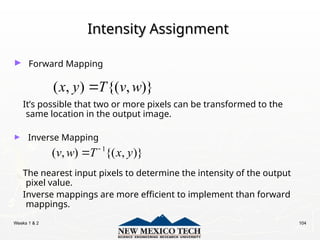
Intensity Assignment
Intensity Assignment
► Forward Mapping
It’s possible that two or more pixels can be transformed to the
same location in the output image.
► Inverse Mapping
The nearest input pixels to determine the intensity of the output
pixel value.
Inverse mappings are more efficient to implement than forward
mappings.
( , ) {( , )}
x y T v w
1
( , ) {( , )}
v w T x y
105.
Weeks 1 &2 105
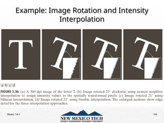
Example: Image Rotation and Intensity
Example: Image Rotation and Intensity
Interpolation
Interpolation
106.
Weeks 1 &2 106
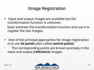
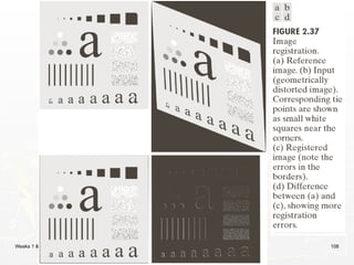
Image Registration
Image Registration
► Input and output images are available but the
transformation function is unknown.
Goal: estimate the transformation function and use it to
register the two images.
► One of the principal approaches for image registration
is to use tie points (also called control points)
The corresponding points are known precisely in the
input and output (reference) images.
107.
Weeks 1 &2 107
Image Registration
Image Registration
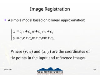
► A simple model based on bilinear approximation:
1 2 3 4
5 6 7 8
Where ( , ) and ( , ) are the coordinates of
tie points in the input and reference images.
x c v c w c vw c
y c v c w c vw c
v w x y
Weeks 1 &2 109
Image Transform
Image Transform
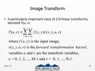
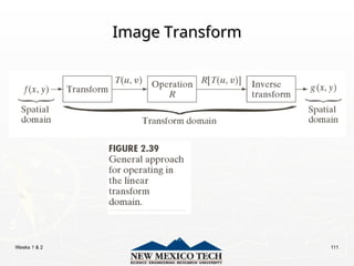
► A particularly important class of 2-D linear transforms,
denoted T(u, v)
1 1
0 0
( , ) ( , ) ( , , , )
where ( , ) is the input image,
( , , , ) is the ker ,
variables and are the transform variables,
= 0, 1, 2, ..., M-1 and = 0, 1,
M N
x y
T u v f x y r x y u v
f x y
r x y u v forward transformation nel
u v
u v
..., N-1.
110.
Weeks 1 &2 110
Image Transform
Image Transform
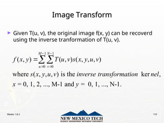
► Given T(u, v), the original image f(x, y) can be recoverd
using the inverse tranformation of T(u, v).
1 1
0 0
( , ) ( , ) ( , , , )
where ( , , , ) is the ker ,
= 0, 1, 2, ..., M-1 and = 0, 1, ..., N-1.
M N
u v
f x y T u v s x y u v
s x y u v inverse transformation nel
x y
Weeks 1 &2 112
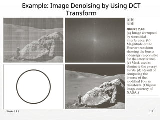
Example: Image Denoising by Using DCT
Example: Image Denoising by Using DCT
Transform
Transform
113.
Weeks 1 &2 113
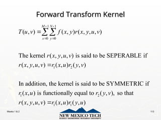
Forward Transform Kernel
Forward Transform Kernel
1 1
0 0
1 2
1 2
( , ) ( , ) ( , , , )
The kernel ( , , , ) is said to be SEPERABLE if
( , , , ) ( , ) ( , )
In addition, the kernel is said to be SYMMETRIC if
( , ) is functionally equal to ( ,
M N
x y
T u v f x y r x y u v
r x y u v
r x y u v r x u r y v
r x u r y v
1 1
), so that
( , , , ) ( , ) ( , )
r x y u v r x u r y u
114.
Weeks 1 &2 114
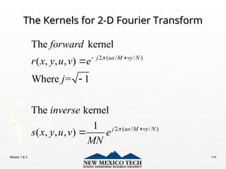
The Kernels for 2-D Fourier Transform
The Kernels for 2-D Fourier Transform
2 ( / / )
2 ( / / )
The kernel
( , , , )
Where = 1
The kernel
1
( , , , )
j ux M vy N
j ux M vy N
forward
r x y u v e
j
inverse
s x y u v e
MN
115.
Weeks 1 &2 115
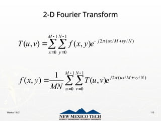
2-D Fourier Transform
2-D Fourier Transform
1 1
2 ( / / )
0 0
1 1
2 ( / / )
0 0
( , ) ( , )
1
( , ) ( , )
M N
j ux M vy N
x y
M N
j ux M vy N
u v
T u v f x y e
f x y T u v e
MN
116.
Weeks 1 &2 116
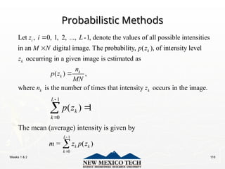
Probabilistic Methods
Probabilistic Methods
Let , 0, 1, 2, ..., -1, denote the values of all possible intensities
in an digital image. The probability, ( ), of intensity level
occurring in a given image is estimated as
i
k
k
z i L
M N p z
z
( ) ,
where is the number of times that intensity occurs in the image.
k
k
k k
n
p z
MN
n z
1
0
( ) 1
L
k
k
p z
1
0
The mean (average) intensity is given by
= ( )
L
k k
k
m z p z
117.
Weeks 1 &2 117
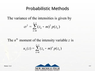
Probabilistic Methods
Probabilistic Methods
1
2 2
0
The variance of the intensities is given by
= ( ) ( )
L
k k
k
z m p z
th
1
0
The moment of the intensity variable is
( ) = ( ) ( )
L
n
n k k
k
n z
u z z m p z
118.
Weeks 1 &2 118
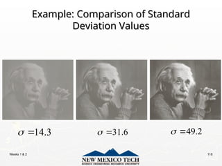
Example: Comparison of Standard
Example: Comparison of Standard
Deviation Values
Deviation Values
31.6
14.3
49.2


![Weeks 1 & 2 42
Representing Digital Images
Representing Digital Images
► Discrete intensity interval [0, L-1], L=2k
► The number b of bits required to store a M × N
digitized image
b = M × N × k](https://image.slidesharecdn.com/lect01-250818190658-b4c489d1/85/Image-processing-and-pattern-recognition-2-ppt-42-320.jpg)


![Weeks 1 & 2 78
Distance Measures
► Given pixels p, q and z with coordinates (x, y), (s, t),
(u, v) respectively, the distance function D has
following properties:
a. D(p, q) ≥ 0 [D(p, q) = 0, iff p = q]
b. D(p, q) = D(q, p)
c. D(p, z) ≤ D(p, q) + D(q, z)](https://image.slidesharecdn.com/lect01-250818190658-b4c489d1/85/Image-processing-and-pattern-recognition-2-ppt-78-320.jpg)
![Weeks 1 & 2 79
Distance Measures
The following are the different Distance measures:
a. Euclidean Distance :
De(p, q) = [(x-s)2
+ (y-t)2
]1/2
b. City Block Distance:
D4(p, q) = |x-s| + |y-t|
c. Chess Board Distance:
D8(p, q) = max(|x-s|, |y-t|)](https://image.slidesharecdn.com/lect01-250818190658-b4c489d1/85/Image-processing-and-pattern-recognition-2-ppt-79-320.jpg)