This document discusses applying a novel approach using multi-criterion decision analysis (MCDA) with the generalized likelihood uncertainty estimation (GLUE) method to quantify uncertainty in hydrological modeling. Specifically, it examines uncertainty in the SLURP hydrological model. Rather than considering overall Nash-Sutcliffe efficiency, the approach considers NSE values for different flow magnitudes simultaneously. The TOPSIS MCDA method is used to compute predictive intervals by considering NSE values for different flow periods simultaneously. The Kootenay Catchment case study is used to demonstrate the MCDA-GLUE approach.

1. 
Abstract—Hydrological models are being used for different
applications. Quantifying the uncertainty of popular
Hydrological models has been well documented, especially with
Bayesian methods such as the Generalized Likelihood
Uncertainty Estimation (GLUE). However, research studies
have often either neglected the lesser known hydrological
models or have performed a typical Bayesian analysis of
uncertainty. In this paper, the SLURP model's uncertainty is
examined using a novel approach of the GLUE method. Instead
of considering the overall Nash Sutcliffe Efficiency (NSE), the
NSE values of different magnitudes of flows are considered
simultaneously to capture the predictive uncertainties of the
SLURP model. By using a Multi-Criterion Decision Analysis
(MCDA) method, the NSE values of different flow periods are
simultaneously considered when computing the predictive
intervals of the SLURP model. Also, the potential issues of using
a MCDA based GLUE approach in lieu of the traditional GLUE
approach are discussed.
Index Terms—TOPSIS, MCDA, bayesian, GLUE.
I. INTRODUCTION
Modeling in Hydrology has expanded beyond traditional
uses and is being utilized over a wide spectrum of
applications. Traditionally, to ensure that the model is
physically representative of the catchment, it is usually
calibrated over a period of time. Following the calibration,
verification of the model is carried out which enables future
use of the model for that catchment. This process was apt
when the basis of application was limited to a stand-alone
usage. Now, hydrological models are employed in
conjunction with other models including atmospheric
models, groundwater models, environmental models, etc.
Therefore it can be concluded that there is a critical need to
understand the nature of the model predictions. This usually
is characterized by performing uncertainty analysis of the
model output.
There are many different methods employed to perform
uncertainty analysis of the model. They are broadly classified
into Bayesian and non-Bayesian methods. One popular
Bayesian method is the Generalized Likelihood Uncertainty
Estimation (GLUE) method. Many researchers have applied
it with valid results, which underscore the versatility and
robustness of the GLUE method [1]-[3]. The GLUE method
is a likelihood estimator based method developed by Beven
Manuscript received March 20, 2014; revised May 21, 2014. This
research was supported by Singapore’s Ministry of Education (MOE) AcRE
Tier 1 Project (M4010973.030) and Tier 2 Project (M4020182.030).
The authors are with the Civil and Environmental Department, Nanyang
Technological University, Singapore 637598 (e-mail:
pramodh1@e.ntu.edu.sg, xsqin@ntu.edu.sg, yuji0011@e.ntu. edu.sg).
and Binley [4] which used Monte Carlo simulation to
quantify uncertainty in a model.
The model used in this study is the SLURP model
developed by Kite [5]. The model has been used by different
studies to model diverse catchments, including large
mountainous catchment [6], wetland [7], etc. Hence, SLURP
is considered as a robust hydrological model. Another
important factor contributing to the decision for choosing
SLURP as the model for this study, is the makeup of the
model parameters. After carrying out analysis, Kite [5]
provides the ten most sensitive parameters that affect the
model accuracy. Hence, this makes it a very useful case to
determine changes in the quantification of parametric
uncertainty when the MCDA method is applied with GLUE.
II. STUDY CASE AND METHODOLOGY
A. Case Study
The Kootenay Catchmentis chosen as the case study to
demonstrate the applicability of MCDA in the GLUE
framework. The mountainous basin which is located in
remote British Columbia, Canada was divided into three
sub-catchments or Aggregated Simulated Areas (ASAs). The
ASAs are Crossing, Canal, and Skookum (outlet of the
waterhsed). The primary land covers of this catchment are
Crop/Grass, Forest and Impervious and the characteristics are
given in Table I.
TABLE I: CHARACTERISTICS OF THE ASAS
Variable Crossing Canal Skookum
Area of ASA (km2
) 411 5040 1790
Mean Elevation (m) 1762 1892 1769
Land Covers
(%)
Impervious 10 9 9
Forest 74 70 62
Crop/Grass 16 21 29
Source: Kite [5]
The SLURP model balances the water budget by dividing
it into four different reservoirs, the canopy storage, the snow
storage, the fast, and slow storage. Further technical details of
the case study are provided in Kite [5]. The ten most sensitive
parameters and their upper and lower bounds are given in
Table II. The calibration process of the model involves 10
years data from 1979 to 1988 (3653 continuous data in a daily
time step). This is followed by a two-year verification period
from 1989 to 1990. The meteorological data for the
corresponding period was obtained from the Canadian Daily
Climate Data [8] and from the CFSR database [9]. The
hydrometric data at the outfalls of the three ASAs were
obtained from Environment Canada’s Hydat database [10].
The topographic information was obtained from Kite [5].
Preliminary Investigation on Coupling MCDA with GLUE
to Perform Uncertainty Analysis of a Hydrological Model
P. Vallam, X. S. Qin, and J. J. Yu
23DOI: 10.7763/IJESD.2015.V6.555
International Journal of Environmental Science and Development, Vol. 6, No. 1, January 2015

2. B. GLUE-MCDA Method
The GLUE method was developed by Beven and Binley
[4]. The underlying principle of this method is that each
parameter ensemble is accorded equal probability of being
representative of the physical processes subsumed in the
SLURP model. Initially, multiple parameter ensembles are
created within their known upper and lower bounds. In this
study, 100,000 such samples were created using the Latin
Hypercube Sampling Scheme to create representative
samples. The set of parameters given in Table II are
replicated for each land-cover and uniform distribution is
used to generate the ensembles. As there are three
land-covers in the Catchment, 300,000 samples were created
with every 30 samples forming a single parameter ensemble.
TABLE II: SENSITIVE PARAMETERS OF SLURP MODEL
Channels
Call
num.
Lower
Bound
Upper
Bound
Initial contents of snow storage
(mm)
P1 1 1000
Initial contents of slow storage (%) P2 0 100
Maximum infiltration rate
(mm/day)
P3 10 100
Manning’s Roughness, n P4 0.0004 0.1
Retention capacity for fast storage
(day)
P5 1 50
Maximum capacity for fast storage
(mm)
P6 10 500
Retention capacity for slow
storage (day)
P7 10 300
Maximum capacity for slow
storage (mm)
P8 100 1000
Precipitation factor P9 0.8 1.5
Rain/snow division temperature
(⁰C)
P10 -2 2
Source: Kite [5]
After identification of the most sensitive parameters, a
suitable likelihood function is chosen. The likelihood
function indicates the performance of the parameter
ensemble during the verification period. In this study, the
commonly used Nash Sutcliffe Efficiency (NSE) is used.
NSE which calculates the accuracy of the model predictions
is commonly used in the applications of the GLUE method
[3].
The threshold level is set at 0.75, which entails that all
parameter ensembles which generate a NSE value greater
than 0.75 is deemed to be physically representative of the
hydrological processes in the Catchment. The successful
values of the parameters maybe further analyzed to determine
their attributes. The model outputs of all the successful
parameters are analyzed by matching the confidence intervals
with the observed flow.
The MCDA method used in this study is the Technique for
Order Preference by Similarity to Ideal Solution (TOPSIS).
This MCDA method was first developed by Hwang and
Yoon [11]. The methodology of TOPSIS entails the
calculation of indices to determine distance from the ideal
solution and the negative ideal solution. Therefore, the best
performing solution would possess the farthest distance to the
negative ideal solution and the shortest distance to the
positive ideal solution. The TOPSIS methodology as detailed
by Triantaphyllou and Lin [12] is employed. In this study, the
flows of the catchment are classified into different categories
and the NSE value for each of the category is calculated for
each parameter ensemble. Then the indices are cutoff at a
point to analyze and compare the flows with the results from
GLUE and with other variations of GLUE-MCDA
methodologies.
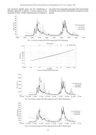
III. RESULTS AND DISCUSSIONS
In the GLUE methodology, the 100,000 parameter
ensembles were run within the SLURP framework using the
Matlab platform. Of the 100,000 parameter ensembles, 4238
different parameter ensembles were considered to have
crossed the threshold. The results from applying the GLUE
methodology are depicted in Fig. 1. The upper bounds of the
confidence interval (CI) are accurate when compared with
the observed flow. The lower bounds of the CI however are
less accurate when compared with the observed flow in the
Kootenay Catchment. Different methodologies instrumented
were chosen to overcome these shortcomings and study the
shifting of the CIs.
A. Methodology I
When applying the GLUE-MCDA method, a critical issue
in the methodology pertains to the classification of flows.
The process to divide the flows into different categories is
arbitrary and requires thorough investigation. The first option
considered entailed carrying out the B17 flood frequency
analysis for the catchment. The HEC-SSP 2.0 software from
the USACE was utilized for this task.
The median plotting positions and the computed
probability curve for the Kootenay Catchment are depicted in
Fig. 2. By using the Return periods of 1, 2 and 10 years, the
flows were classified into different categories. The different
categories were flows <400 m3
/sec, 400-640 m3
/sec, 640-867
m3
/sec and >867 m3
/sec. The NSE value for each category
was calculated and finally, the TOPSIS procedure was
performed to develop the indices. Equal weight age was
given for all the flow categories. The ideal solution was
considered to be the maximum NSE value for each category
and the non-ideal solution was the minimum NSE value for
the same category. To ensure parity when comparing the
outcomes of the GLUE-MCDA and just the GLUE
methodology, equal width in the TOPSIS index and the
likelihood function was considered. The maximum and
minimum overall NSE values were -0.2985 and 0.8291
respectively. With these values, the distance to the threshold
value of 0.75 was calculated to be 0.0702. Similarly, the
minimum and the maximum value of the calculated TOPSIS
index were examined and the same procedure performed to
arrive at the new cutoff point. With a minimum and
maximum TOPSIS index for the segmented NSE values
being 0.3969 and 0.9048, the cutoff point was computed to be
0.8692. This yielded the top 6 values for further analysis. The
confidence intervals of these predictions were calculated and
subsequently plotted in Fig. 3. The results presented a
significant savings in the time required for computation when
compared to the GLUE methodology (Fig. 1). However, the
TOPSIS method performed in this manner compromised on
the accuracy of the Confidence Intervals of the flow,
especially for the first year. The difference in the nature of the
hydrographs for the two years played an important role in the
output of the methodology. The hydrograph for the second
24
International Journal of Environmental Science and Development, Vol. 6, No. 1, January 2015

3. year possessed multiple peaks and this methodology is
definitely applicable to perform a cursory analysis on the
uncertainty in flows. Another important point of similarity in
the results is the comparable magnitudes of the lower bounds
for both the results and the observed flow during the low flow
periods.
0
100
200
300
400
500
600
700
800
900
32400 32500 32600 32700 32800 32900 33000 33100 33200 33300
Flow(m3/sec)
Observed Flow
Lower Bounds
Upper Bounds
Fig. 1. CI of the flows during 1989-1990 by applying the GLUE methodology.
Fig. 2. B17 Plot for the Kootenay basin.
0.00
200.00
400.00
600.00
800.00
1000.00
1200.00
14/9/1988 23/12/1988 2/4/1989 11/7/1989 19/10/1989 27/1/1990 7/5/1990 15/8/1990 23/11/1990 3/3/1991
Flow(m3/sec)
Observed Flows
Lower Bounds
Upper Bounds
Fig. 3. CI of the flows during 1989-1990 by applying the GLUE-MCDA Methodology I.
0.00
100.00
200.00
300.00
400.00
500.00
600.00
700.00
800.00
900.00
14/9/1988 23/12/1988 2/4/1989 11/7/1989 19/10/1989 27/1/1990 7/5/1990 15/8/1990 23/11/1990 3/3/1991
Flow(m3/sec)
Observed Flow
Lower Bounds
Upper Bounds
Fig. 4. CI of the flows during 1989-1990 by applying the GLUE-MCDA Methodology II.
25
International Journal of Environmental Science and Development, Vol. 6, No. 1, January 2015

4. B. Methodology II
Following this, the flow categories were rationalized to
ensure improvements over the previous methodology. The
categories were adjusted to equally represent the different
magnitudes in the flows observed in Kootenay Catchment.
The categories then adopted were <100 m3
/sec, 100-250
m3
/sec, 250-450 m3
/sec, 450-600 m3
/sec and >600 m3
/sec.
The NSE values were given equal weights of 0.2 when
TOPSIS methodology was performed. As with the earlier
case, the indices were computed and the equal width was
used as the cutoff point. The highest and the lowest TOPSIS
indices were 0.9419 and 0.4225. The output from the top
7130 parameter ensembles were then selected to generate the
Confidence Intervals. Fig. 4 depicts the CI for the flows
generated in this manner.
The CI from this methodology presented an improvement
over the results from the previous methodology. The CI of the
peak flows during the first year is more balanced when
compared to the GLUE methodology (Fig. 1) and previous
methodology (Fig. 3). This is of critical importance when the
magnitude of the upper bound is closer to the actual flow.
This would make this methodology more suitable for future
modifications of the river flow based on the peak availability.
However, the drawback of this method manifests when the
peak flows of the second year are examined. The SLURP
model predicts hydrographs of a single major peak more
accurately than hydrographs with multiple peaks for this
watershed. This is most evident in the current methodology
where the categorization of flows pre-disposes the accuracy
of the flows towards flows of lower magnitudes.
0.00
100.00
200.00
300.00
400.00
500.00
600.00
700.00
800.00
900.00
14/9/1988 23/12/1988 2/4/1989 11/7/1989 19/10/1989 27/1/1990 7/5/1990 15/8/1990 23/11/1990 3/3/1991
Flow(m3/sec)
Observed Flow
Lower Bounds
Upper Bounds
Fig. 5. CI of the flows during 1989-1990 by applying the GLUE-MCDA Methodology III.
0.00
100.00
200.00
300.00
400.00
500.00
600.00
700.00
800.00
900.00
14/9/1988 23/12/1988 2/4/1989 11/7/1989 19/10/1989 27/1/1990 7/5/1990 15/8/1990 23/11/1990 3/3/1991
Flow(m3/sec)
Observed Flow
Lower Bounds
Upper Bounds
Fig. 6. CI of the flows during 1989-1990 by applying the GLUE-MCDA Methodology IV with weights 0.33, 0.33, and 0.34.
0.00
100.00
200.00
300.00
400.00
500.00
600.00
700.00
800.00
900.00
14/9/1988 23/12/1988 2/4/1989 11/7/1989 19/10/1989 27/1/1990 7/5/1990 15/8/1990 23/11/1990 3/3/1991
Flow(m3/sec)
Observed Flow
Lower Bounds
Upper Bounds
Fig. 7. CI of the flows during 1989-1990 by applying the GLUE-MCDA Methodology IV with weights 0.1, 0.1, and 0.8.
26
International Journal of Environmental Science and Development, Vol. 6, No. 1, January 2015

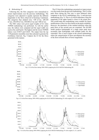
5. C. Methodology III
Another aspect of the methodology to understand the
variations of the CI of the flows is to quantify the influence of
the overall NSE within the TOPSIS framework. Uncertainty
quantification by computing and further analyzing the CI of
the flows can be modified to suit the research purposes. In
this part of the GLUE-MCDA methodology, the overall NSE
is accorded a weighing factor of 0.3 and the different
categories are accorded a weighing factor of 0.15. The
exception was the >600 m3
/sec category which was accorded
a weighing factor of 0.1 on the account that only a few
periods of flows were modeled in this category. Based on
maximum and minimum TOPSIS index values of 0.9385 and
0.4173, the cutoff point was 0.8837 which resulted in the top
36171 parameter ensembles performing. The CI of the flows
(Fig. 5) depicts the reduction of magnitudes of the upper limit
of the CI during the peak of the first year. During the low
flow periods, the model generally tended to predict flows
greater than the observed flow. This property of the SLURP
model was observed when performing analyses with all the
different versions of the methodologies. This may be
attributed to the model structure that predisposes predictions
towards lagging in output.
D. Methodology IV
After examining the results from the previous two
methodologies, it can be concluded that the GLUE-MCDA
methodology is quite sensitive to the categorization of the
flows. Another aspect of the methodology that affects the
accuracy is the weights accorded to the NSE of each
category. To further rationalize the flow categories, the
magnitudes were divided into low flow, medium flow and
peak flow. The categories were <100 m3
/sec, 100-350 m3
/sec
and >350 m3
/sec. To study the influence of the weights
accorded to the NSE of each category, weights of 0.33, 0.33
and 0.34 were initially accorded to each category. Following
this, a weight of 0.8 was accorded to one category and 0.1 to
the other categories. Altering of weights for each category
can typify the shifting of CIs of flows predicted in a typical
uncertainty analyses.
The 100,000 parameter ensembles were run with the
weights 0.33, 0.33 and 0.34 and the TOPSIS indices
calculated. Based on the principle of equal width, the cutoff
point for the TOPSIS indices was computed as 0.9136. This
yielded 25221 best performing samples. The CIs of these
flows were computed and plotted in Fig. 6. The magnitudes
of the upper bounds in the results depicted by Fig. 6
demonstrate significantly better performance for the first year
when compared to the GLUE methodology. The two most
significant improvements is the reduction in magnitudes of
the upper CI limits and the non-exceedence of the lower CI
limits during the peak flow periods. However, as the CI width
of this period is narrower when the GLUE methodology is
applied, the application of the GLUE methodology is
considered to be more appropriate. During the second year,
the CIs of the flows were shown to under-predict for the
catchment. This can be attributed to the majority of the flows
in the 730 time steps (2 years) belonging to the low flow
period.
The weights of 0.8 for low flow period and weights of 0.1
and 0.1 were assigned to the medium and high flow periods.
Based on the principle of equal width, the cutoff point for the
TOPSIS indices was computed as 0.8962 (which yielded the
top 33197 ensembles). Similarly the cutoff points were
0.8982 when medium flow was accorded 0.8 (yielding 67056
ensembles) and 0.9010 when high flow was accorded 0.8
(yielding 65452 ensembles). The results of these three
different variations of the methodology yielded expected
results. There was an increase in the magnitudes of the upper
bounds of the CI of the peak flows when the high flow was
accorded 0.8 (Fig. 7). However significant change in the
lower bounds of the CI was noticed during the peak flow
period. The upper bounds of the CI for the second year were
observed to be closer to the observed flow when high flow
was accorded a weight of 0.8, making this methodology more
appropriate for studies focusing on the peak flow events in
the catchment. For studies focusing on the low flow periods,
such as irrigation or drought management studies, assigning
low flow category with a weight higher than 0.8 may be more
suitable to obtain a weighed and balanced view of the
catchment.
IV. CONCLUSIONS
The different methodologies discussed in the previous
section illustrate the various directions in which the
GLUE-MCDA methodology may be applied. The final
results present potential improvements in certain aspects of
the flows over the different variations of the methodology.
However, the results from the GLUE methodology are
considered to be more accurate, especially when the second
year is considered. An attempt to investigate the salient
factors that affect the accuracy of the overall framework has
been documented. By suitably modifying this methodology,
uncertainty quantification focusing on the different aspects of
hydrologic modeling can be conducted, enhancing the role of
MCDA methods in traditional uncertainty analyses. The most
suitable and comparable result of the methodology would
usually require the inclusion of the overall NSE. Moreover,
from the results obtained, it can be judged that the results
based solely on the different categories may still yield less
accurate results when compared to the GLUE methodology.
Furthermore, including the GLUE technique within the
MCDA framework demonstrates potential to enhance the
validity of the uncertainty analyses, modifications to the
MCDA framework beyond the flow categories maybe
essential.
REFERENCES
[1] Z. Y. Shen, L. Chen, and T. Chen, “Analysis of parameter uncertainty
in hydrological and sediment modeling using GLUE method: A case
study of SWAT model applied to Three Gorges Reservoir Region,
China,” Hydrol. and Earth Sys. Sci., vol. 16, no. 1, pp. 121-132,
January 2012.
[2] A. Montanari, “Large sample behaviors of the generalized likelihood
uncertainty estimation (GLUE) in assessing the uncertainty in
rainfall-runoff simulations,” Water Resour. Research, vol. 41, no. 8,
pp. 1-13, August 2005.
[3] J. R. Stedinger, R. M. Vogel, S. U. Lee, and R. Batchelder, “Appraisal
of the generalized likelihood uncertainty estimation,” in Proc. World
Environment and Water Resources Congress, Honolulu, May 2008,
pp. W00B06-1-W00B06-17.
[4] K. Beven and A. Binley, “The future of distributed models: Model
calibration and uncertainty prediction,” Hydrol. Processes, vol. 6, no.
3, pp. 279-298, July/September 1992.
27
International Journal of Environmental Science and Development, Vol. 6, No. 1, January 2015

6. [5] G. W. Kite, Manual for the SLURP Hydrological Model V. 11,
Saskatoon, Canada: NHRC, 1997.
[6] R. Thorne and M. K. Woo, “Efficacy of a hydrologic model in
simulating discharge from a large mountainous catchment,” Journal of
Hydrol., vol. 330, no. 1-2, pp. 301-312, October 2006.
[7] K. D. Voogt, G. W. Kite, P. Droogers, and H. Murray-Rust, “Modeling
water allocation between a wetland and irrigated agriculture in the
Gediz Basin, Turkey,” Intl. Journal of Water Resour. Develpmt., vol.
16, no. 4, pp. 639-650, 2000.
[8] National Climate Data and Information Archive. (2014). Historical
climate data-environment Canada, Gatineau, QC. [Online]. Available:
http://weather.gc.ca/
[9] National Centers for Environmental Prediction (NCEP) Climate
Forecast System Reanalysis (CFSR). (2013). Global Weather for
SWAT. [Online]. Available: http://globalweather.tamu.edu/
[10] National Water Data Archive. (2012). HYDAT archived hydrometric
data, environment Canada, Gatineau, QC. [Online]. Available:
http://www.wsc.ec.gc.ca/applications/H2O/index-eng.cfm
[11] C. L. Hwang and K. Yoon, Multiple Attribute Decision Making:
Methods and Applications, New York: Springer-Verlag, 1981.
[12] E. Triantaphyllou and C. T. Lin, “Development and evaluation of five
fuzzy Multiattribute decision-making methods,” Intl. Journal of
Approx. Reasoning, vol. 14, no. 4, pp. 281-310, May 1996.
Pramodh Vallam received M.S. degree in
environmental engineering from Stanford University
and Nanyang Technological University, Singapore in
2010.
He is currently a Ph.D. candidate in environment
and water resources engineering in Nanyang
Technological University. He is working on the
application of hydrological models to model
large-scale watersheds. He was a project officer with
the DHI-NTU Water & Environment Research Center and Education Hub,
DHI Water & Environment (S) Pte. Ltd., working on a sustainability project
for the Nanyang Technological University. His research focuses on
hydrology, water resources planning, uncertainty quantification and impact
of climate change on large-scale watersheds.
Xiaosheng Qin received Ph.D. degree in environment
system engineering from University of Regina,
Canada in 2008.
He is an assistant professor at the Nanyang
Technological University, Singapore. His research
focuses on water resources planning, hydrologic
modeling, climate change impact assessment,
groundwater modeling, urban air quality and solid
waste management.
Dr. Qin was awarded the Young Scientist Paper Award (Third Place) at
the 6th International Conference on Environmental Science and Technology
2012, Houston, USA, and also awarded the Best Practice-Oriented Paper
Award (American Society of Civil Engineers) from Environmental
Multi-Media Council, World Water & Environmental Resources Congress,
Salt Lake City, Utah, USA in June 2004. He is an associate member of
ASCE, member of ISEIS, IWA and IAHR.
Jianjun Yu received M.Sc. degree in geographic
information system in Zhejiang University, China in
2005.
He is currently a researcher in DHI-NTU Water &
Environment Research Center and Education Hub,
DHI Water & Environment (S) Pte. Ltd. His research
focuses on hydrology, hydraulics, water resources
planning and watershed management, uncertainty
analysis, flood and environmental risk management,
application of geographic information system and remote sensing techniques
in environment and water resources fields.
28
International Journal of Environmental Science and Development, Vol. 6, No. 1, January 2015