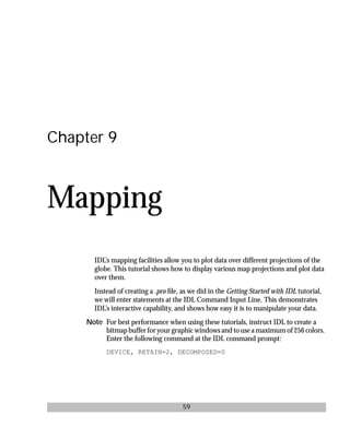
This document introduces the basics of IDL, including its interactive and programming capabilities. IDL allows array-oriented processing and visualization of data. Simple IDL commands can perform powerful tasks like arithmetic, plotting, image processing, and more. The tutorials provide hands-on examples of common IDL applications like 2D/3D plotting, reading/writing data, animation, and more. Users can explore data interactively and create complete applications by writing IDL programs.

![basics.bk : power.doc 4 Mon Apr 28 12:26:12 1997
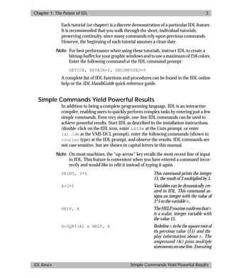
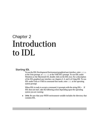
4 Chapter 1: The Power of IDL
Simple Commands Yield Powerful Results IDL Basics
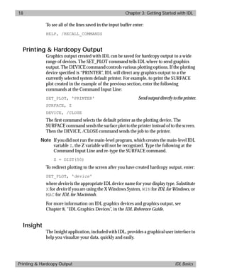
the SQRT command makes A a
floating-point variable.
A = [1, 2, 3, 4, 5, 6] Make A a 6-element array con-
taining the integer values 1
through 6.
PRINT, A, 2*A IDL operators and functions work
on both scalar and array data
types with no change in notation.
B = SQRT(A) Take the square root of each ele-
ment of array A and put those val-
ues into the variable B.
HELP, A, B Show that A and B are arrays of 6
dimensions. The elements of A are
integerswhiletheelementsofB are
floating-point values.
PRINT, B Display the 6 floating-point ele-
ments in array B.
A = FLTARR(100) Define A as an array of 100 float-
ing-point elements.
FOR i = 0,99 DO A[i] = i This FOR loop stores in each ele-
mentofA thevalueofitssubscript.
Forexample,thevalueofA[0]=0
and A[40]=40.
PRINT, A[0], A[99] IDLsubscriptsbeginat0andgoto
one less than the number of ele-
ments. This command prints the
first and last elements of our 100-
element array.
PRINT, A[10:19] Subarrays can be specified by us-
ing subscript ranges. This com-
mand prints the values of A[10]
through A[19].
B = SIN(A/5)/EXP(A/50) Create a 100-element floating-
point vector describing a damped
sine wave.
PLOT, B Make a two-dimensional plot of
the vector B.
PLOT, B, COS(A/5) Plot the vector B versus the vector
described by the cosine of (A/5).](https://image.slidesharecdn.com/idlbasics-190222151049/85/Idl-basics-10-320.jpg)


![basics.bk : 2d.doc 24 Mon Apr 28 12:26:12 1997
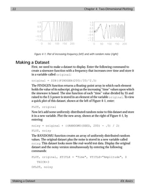
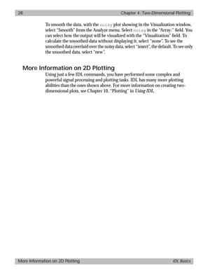
24 Chapter 4: Two-Dimensional Plotting
Displaying the Results IDL Basics
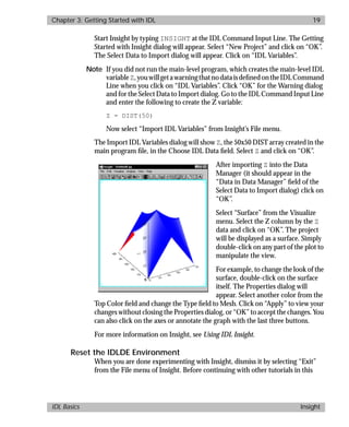
Y[101:199] = - REVERSE(Y[1:99]) Make the last 99 elements of Y a
mirror image of the first 99 ele-
ments.
filter = 1.0 / (1 + (Y/40)^10) Create a variable filter to hold
the filter function based on Y.
PLOT, filter Plot a fifth-order Butterworth fil-
terwithacutoffof40cyclesperto-
tal sampling period,.
To filter data in the frequency domain, we multiply the Fourier transform of the
data by the frequency response of a filter and then apply an inverse Fourier
transform to return the data to the spatial domain. Now we can use a lowpass
filter on the noisy dataset and store the filtered data in the variable lowpass by
entering:
lowpass = FFT(FFT(noisy, 1) * filter, -1)
PLOT, lowpass
The same filter function can be used as a high-pass filter (allowing only the high
frequency or noise components through) by entering:
highpass = FFT(FFT(noisy, 1) * (1.0 - filter), -1)
PLOT, highpass
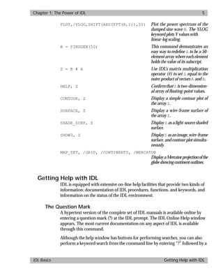
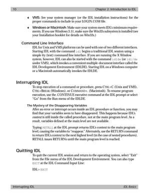
Displaying the Results
Now let’s look at all of the results at the same time. We can split the plotting
window into six sections, and make each section display a different plot. The
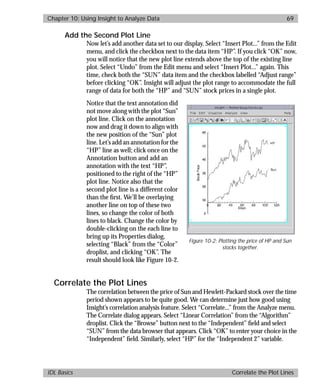
system variable !P.MULTI tells IDL how many plots to put on a single page.
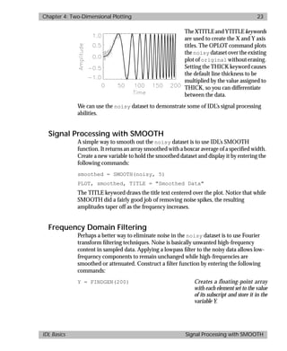
Enter the following lines to display the plotting window shown in Figure 4-2.
!P.MULTI = [0,2,3] Display all plots at the same time
with 2 columns and 3 rows.
PLOT, original, TITLE = 'Original "Ideal" Data'
Display original dataset, upper
left.
PLOT, noisy, TITLE="Noisy Data" Displaynoisydataset,upperright.
PLOT, SHIFT(FILTER, 100), TITLE = "Filter Function"
Displayfilterfunction,middleleft.
The SHIFT function was used to
show the filter’s peak as centered.](https://image.slidesharecdn.com/idlbasics-190222151049/85/Idl-basics-30-320.jpg)
![basics.bk : 2d.doc 26 Mon Apr 28 12:26:12 1997
26 Chapter 4: Two-Dimensional Plotting
Plotting with Missing or Bad Data IDL Basics
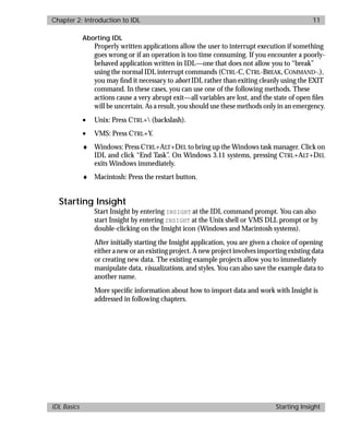
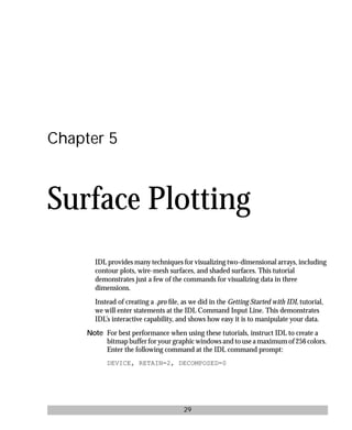
Plotting with Missing or Bad Data
The PLOT routine can be used to easily create plots where values for some data
points are missing.
Suppose that you have a dataset that contains “bad” values. For example, a device
that measures sun intensity may produce meaningless data when a cloud
obscures its view. To simulate such a dataset, enter the following commands from
the IDL prompt:
A = INDGEN(50)
A[RANDOMU(SEED, 10) * 50] = 999
The first command creates a 50-element array where each element is set to the
value of its subscript (i.e., the value of A[0] is 0, the value of A[30] is 30). The
second command sets the values of ten randomly selected points to the “bad”
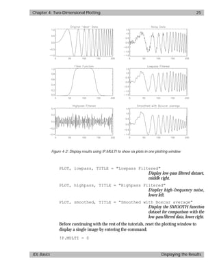
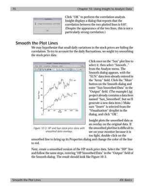
value, 999. Display this dataset, the plot at the left of Figure 4-3, with the PLOT
command:
PLOT, A
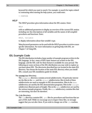
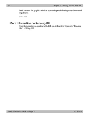
The problem is immediately apparent. The bad data values cause the plot to be
scaled such that the good data values can hardly be read. Using the MAX_VALUE
keyword to PLOT, we can avoid plotting the noise values and scale the good data
values accordingly.
The MAX_VALUE keyword is set to the largest data value to be plotted. Data
larger than this value are treated as missing data and are not plotted. Create the
missing data plot of A, the plot at the right of Figure 4-3, by entering:
PLOT, A, MAX_VALUE=998
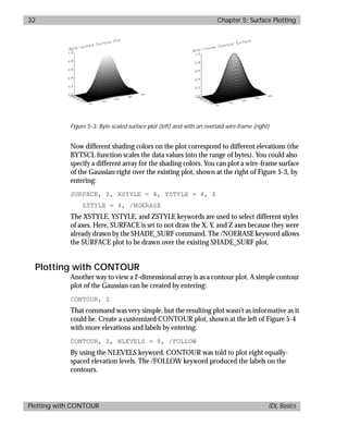
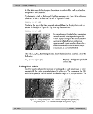
Figure 4-3: Plot with “bad” values (left) and plot using MAX_VALUE (right)](https://image.slidesharecdn.com/idlbasics-190222151049/85/Idl-basics-32-320.jpg)


![basics.bk : image.doc 44 Mon Apr 28 12:26:12 1997
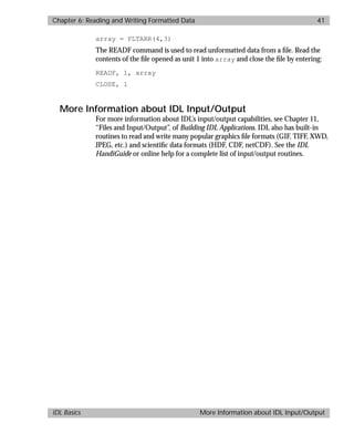
44 Chapter 7: Image Processing
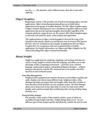
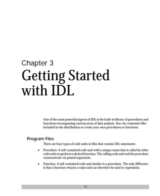
Reading an Image IDL Basics
Reading an Image
First we must import an image to be processed. Reading data files into IDL is easy
if you know the format in which the data is stored. Often, images are stored as
arrays of bytes. The file that we will read contains an image of an aerial view above
New York City stored as a byte array.
Opening an Image File
Open the file for reading by entering:
OPENR, 1, FILEPATH('nyny.dat', SUBDIR = ['examples', 'data'])
The OPENR statement opens the file named in quotes for reading and assigns it
the logical unit number listed as the first argument to the OPENR statement. Here
we assign the file nyny.dat to unit number 1. The file is subsequently referred
to by using the logical unit number. Unit numbers can range from 1 to 128. The
FILEPATH function, used as an argument to OPENR, returns the full path for the
file nyny.dat located in the data subdirectory of the examples
subdirectory of the IDL distribution.
Images as Arrays of Data
When images are stored as multiple arrays of unformatted binary data, it is
convenient to use the ASSOC function to establish an association between a
sequence of arrays and the data file. The image in the file nyny.dat is a 768-
element by 512-element array of bytes, so we will associate the resulting
rectangular array called A with file unit number 1 by entering:
A=ASSOC(1, BYTARR(768, 512))
Now A[0] corresponds to the first 768 by 512-byte image in the file nyny.dat,
which happens to be the only image. You can include several images in a file. For
example, the third image in a file, after being extracted exactly as described above,
is specified as A[2].
B=A[0] Read the image into variable B.
CLOSE, 1 Close the file.
Note Every reference to A[0] rereads the image from disk. To hold the file in
memory, store it in the memory-resident array B.
Displaying an Image
You can view an image in IDL with two different routines. The TV procedure
writes an array to the display as an image without scaling. The TVSCL procedure](https://image.slidesharecdn.com/idlbasics-190222151049/85/Idl-basics-50-320.jpg)
![basics.bk : image.doc 50 Mon Apr 28 12:26:12 1997
50 Chapter 7: Image Processing
Other Image Manipulations IDL Basics
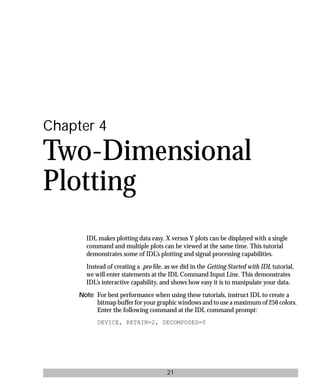
Another commonly used gradient operator is the Sobel operator. IDL’s SOBEL
function operates over a 3 by 3 region, making it less sensitive to noise than some
other methods. Enter the following:
SO=SOBEL(B) Create a Sobel sharpened version
of the image.
TV, SO Display the sharper image.
Other Image Manipulations
Sections of images can be easily displayed by using subarrays. Erase the current
display, create a new array that contains Upper New York Bay and display it by
entering:
ERASE
E = B[100:300, 150:250]
TV, E
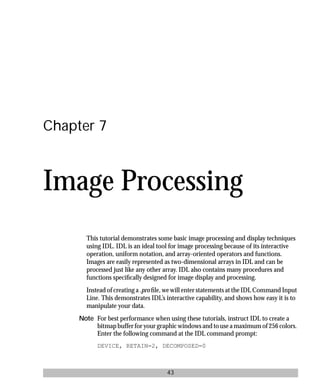
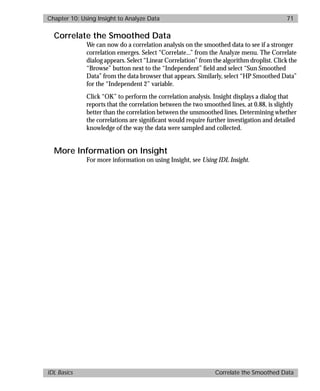
Resizing with CONGRID
Resize Upper New York Bay using CONGRID. Unlike the REBIN command,
CONGRID can resize arrays to any arbitrary size. Set each dimension of E to 500
elements and display the result, as shown at the left of Figure 7-5, by entering:
E = CONGRID(E, 500, 500, /INTERP)
TV, E
The /INTERP keyword causes bilinear interpolation to be used.
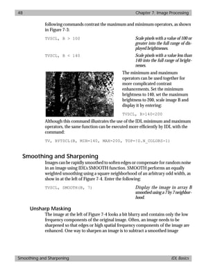
Figure 7-5: Using CONGRID to resize an image (left) and Rotating an image (right)](https://image.slidesharecdn.com/idlbasics-190222151049/85/Idl-basics-56-320.jpg)

![basics.bk : grid.doc 57 Mon Apr 28 12:26:12 1997
Chapter 8: Plotting Irregularly-Gridded Data 57
IDL Basics The TRIANGULATE Procedure
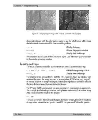
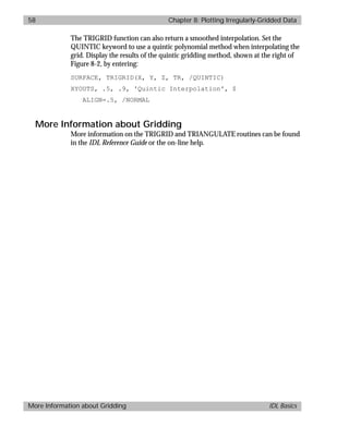
The TRIANGULATE Procedure
The TRIANGULATE procedure constructs a Delaunay triangulation of a planar
set of points. After a triangulation has been found for a set of irregularly-gridded
data points, the TRIGRID function can be used to interpolate surface values to a
regular grid.
To return a triangulation in the variable TR, enter the command:
TRIANGULATE, X, Y, TR
The variable TR now contains a 3-element by 54-element longword array. To
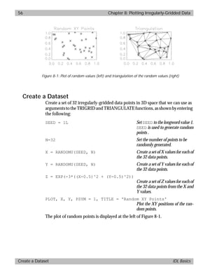
produce a plot of the triangulation, shown at the right of Figure 8-1, enter the
following commands:
PLOT, X, Y, PSYM = 1, TITLE = 'Triangulation'
FOR i=0, N_ELEMENTS(TR)/3 - 1 DO BEGIN & $
T = [TR[*, i], TR[0, i]] & $
PLOTS, X[T], Y[T] & ENDFOR
Plotting the Results with TRIGRID
Now that we have the triangulation TR, the TRIGRID function can be used to
return a regular grid of interpolated Z values.
Display a surface plot of the gridded data using the default interpolation
technique and add a title to the plot, shown at the left of Figure 8-2, by entering:
SURFACE, TRIGRID(X, Y, Z, TR)
XYOUTS, .5, .9, 'Linear Interpolation', $
ALIGN=.5, /NORMAL
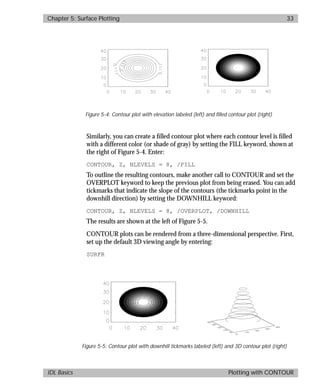
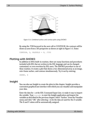
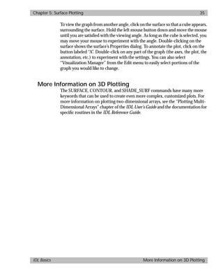
Figure 8-2: Linear interpolation of triangulated data (left) and Quintic interpolation (right)](https://image.slidesharecdn.com/idlbasics-190222151049/85/Idl-basics-63-320.jpg)
![basics.bk : map.doc 61 Mon Apr 28 12:26:12 1997
Chapter 9: Mapping 61
IDL Basics Drawing an Orthographic Projection
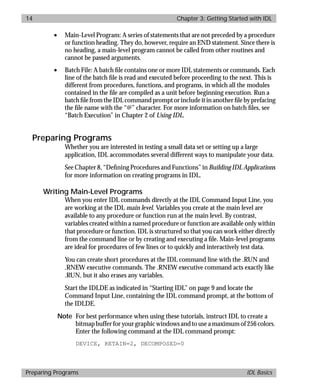
MAP_CONTINENTS, COLOR = 220, /FILL Draw the continent outlines. The
FILL keyword fills in the conti-
nents using the color specified by
the COLOR keyword.
MAP_GRID, COLOR = 160, /LABEL Draw the grid lines. The COLOR
keyword specifies the color of the
gridlines.TheLABELkeywordla-
bels the lines.
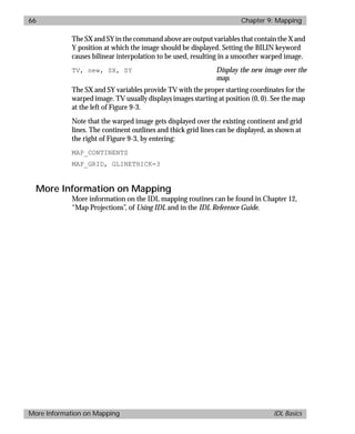
The order of MAP_GRID and MAP_CONTINENTS depends on how you wish
to display your map. In the above example, if you call MAP_GRID before
MAP_CONTINENTS, the filled continents are drawn over the labeled grid lines.
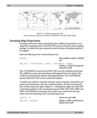
Drawing an Orthographic Projection
To draw a map that looks more like a globe, use the orthographic projection.
Enter the following at the Command Input Line:
MAP_SET, 30, -100, 0, /ORTHO, /ISOTROPIC, /GRID, $
/CONT, /LABEL, /HORIZON
The orthographic projection to the left shows
North America at the center.
ThenumbersfollowingtheMAP_SETcommand(30,-
100,and0)arethelatitudeandlongitudetobecentered
and the angle of rotation for the North direction. The
ISOTROPIC keyword creates a map that has the same
scale in the vertical and horizontal directions, so we get
acircularmapinarectangularwindow.Notethatwe’ve
abbreviatedtheCONTINENTSkeywordtoCONTand
the ORTHOGRAPHIC keyword to ORTHO. IDL keywords (but not function and
procedure names) can always be abbreviated to their minimum unique length. The
GRID, COLOR, and LABEL keywords work the same as before. The HORIZON
keyword draws the line at which the horizon exists. Without the HORIZON keyword,
MAP_SET only draws the grid and the continents.
Plotting a Portion of the Globe
You don’t always have to plot the entire globe. The LIMIT keyword specifies a
region of the globe to plot. Enter the following at the Command Input Line:
MAP_SET, 32, -100, /AZIM, LIMIT=[10, -130, 55, -70], /GRID, $
/CONT, /LABEL](https://image.slidesharecdn.com/idlbasics-190222151049/85/Idl-basics-67-320.jpg)
![basics.bk : map.doc 62 Mon Apr 28 12:26:12 1997
62 Chapter 9: Mapping
Plotting Data on Maps IDL Basics
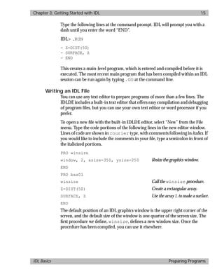
The azimuthal equidistant projection to
the left shows the United States and
Mexico. The AZIM keyword selects the
azimuthal equidistant projection. The
keyword LIMIT is set equal to a four-
element vector containing the minimum
latitude, minimum longitude, maximum
latitude, and maximum longitude.
You can also limit the section of the map you are viewing by using the SCALE
keyword, which constructs an isotropic map with the given scale, set to the ratio
of 1:scale at the center of the map. If SCALE is not specified, the map is fit to the
window.
Plotting Data on Maps
You can annotate plots easily in IDL. To plot the location of selected cities in
North America, as shown at the left of Figure 9-2, you need to create three arrays:
one to hold latitudes, one to hold longitudes, and one to hold the names of the
cities being plotted. Enter the following at the Command Input Line:
LATS = [40.02, 34.00, 38.55, 48.25, 17.29]
Create a 5-element array of float-
ing-point values representing lati-
tudes in degrees North of zero.
LONS = [-105.16, -119.40, -77.00, -114.21, -88.10]
The values in LONS are negative
because they represent degrees
West of zero longitude.
CITIES = ['Boulder, CO', 'Santa Cruz, CA', $
'Washington, DC', 'Whitefish, MT', 'Belize, Belize']
Create a five-element array of
string values. Text strings can be
enclosed in either single quotes
('text') or double quotes ("text").
MAP_SET, /MERCATOR, /GRID, /CONTINENT, $
LIMIT = [10, -130, 60, -70] Draw a Mercator projection fea-
turing the United States and
Mexico.](https://image.slidesharecdn.com/idlbasics-190222151049/85/Idl-basics-68-320.jpg)
![basics.bk : map.doc 64 Mon Apr 28 12:26:12 1997
64 Chapter 9: Mapping
Plotting Contours Over Maps IDL Basics
Plotting Contours Over Maps
Contour plots can easily be drawn over map projections by using the OVERPLOT
keyword to the CONTOUR routine. See the map at the right of Figure 9-2. Enter
the following at the Command Input Line:
A = DIST(91) Create a dataset to plot.
LAT = FINDGEN(91) * 2 - 90 Create an X value vector contain-
ing 91 values that range from -90
to 90 in 2 degree increments.
LON = FINDGEN(91) * 4 - 180 Createa Yvaluevector containing
91 values that range from -180 to
180 in 4 degree increments.
MAP_SET, /GRID, /CONTINENTS, /SINUSOIDAL, /HORIZON
Create a new sinusoidal map pro-
jectionoverwhichtoplotthedata.
CONTOUR, A, LON, LAT, /OVERPLOT, NLEVELS = 12
Draw a twelve-level contour plot
of array A over the map.
Since latitudes range from -90 to 90 degrees and longitudes range from -180 to
180 degrees, you created two vectors containing the “X” and “Y” values for
CONTOUR to use in displaying the array A. If the X and Y values are not
explicitly specified, CONTOUR will plot the array A over only a small portion of
the globe.
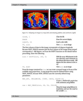
Warping Images to Maps
Image data can also be displayed on maps. The MAP_IMAGE function returns a
warped version of an original image that can be displayed over a map projection.
In this example, elevation data for the entire globe is displayed as an image with
continent outlines and grid lines overlaid. Enter the following at the Command
Input Line:
OPENR, 1, FILEPATH('worldelv.dat', SUB=['examples', 'data'])
Open the elevation data file,
worldelv.dat. This file contains a
360-element square array of byte
values.
elev = BYTARR(360, 360) Create the appropriately-sized
byte array.
READU, 1, elev Readthedatafromthefileintothe
variable elev.](https://image.slidesharecdn.com/idlbasics-190222151049/85/Idl-basics-70-320.jpg)

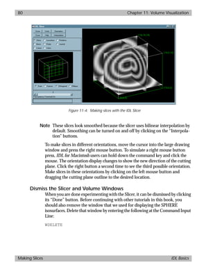
![basics.bk : volume.doc 75 Mon Apr 28 12:26:12 1997
Chapter 11: Volume Visualization 75
IDL Basics Create a Dataset
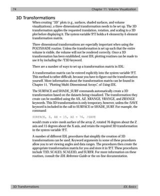
Create a Dataset
Open a new editor window as described in “Writing an IDL File” on page 15.
You will create a 3D volume dataset that has 20 elements in each of the X, Y, and
Z directions. The value of each point within the volume is equal to that point’s
distance from the center of the volume, point (10, 10, 10). Write the following in
the editor window:
PRO sphere
WINDOW, 0, XSIZE=600, YSIZE=600 Make a square graphics window.
SPHERE = FLTARR(20, 20, 20)
FOR X=0,19 DO BEGIN
FOR Y=0,19 DO BEGIN
FOR Z=0,19 DO SPHERE[X, Y, Z] = $
SQRT((X-10)^2+(Y-10)^2+(Z-10)^2)
ENDFOR
ENDFOR
The first command creates an empty, floating-point array. The three nested FOR
loops of the second command compute the value of each point within the array.
In this array, all points with the same value are at approximately the same
distance from the center of the volume. Each constant-density surface (iso-
surface) is roughly spherical.
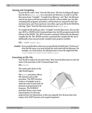
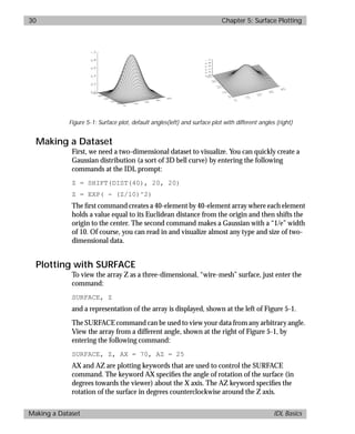
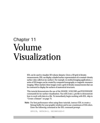
Visualizing an Iso-Surface
Two IDL commands, SHADE_VOLUME and
POLYSHADE, are used together to visualize an iso-
surface. SHADE_VOLUME generates a list of polygons
that define a 3D surface given a volume dataset and a
contour (or density) level. The procedure POLYSHADE
can then be used to create a shaded-surface
representation of the iso-surface from those polygons,
shown to the left.
Like many other IDL commands, POLYSHADE accepts the T3D keyword that
makes POLYSHADE use a user-defined 3D transformation. Before you can use
POLYSHADE to render the final image, you need to set up an appropriate three-
dimensional transformation, described in more detail in “3D Transformations”
on page 74. The XRANGE, YRANGE, and ZRANGE keywords accept 2-element](https://image.slidesharecdn.com/idlbasics-190222151049/85/Idl-basics-81-320.jpg)
![basics.bk : volume.doc 76 Mon Apr 28 12:26:12 1997
76 Chapter 11: Volume Visualization
A More Complex Dataset IDL Basics
vectors, representing the minimum and maximum axis values, as arguments.The
POLYSHADE function returns an image based upon the list of vertices, V, and list
of polygons, P. The /T3D keyword tells POLYSHADE to use the previously-
defined 3D transformation. The TV procedure displays the shaded-surface
image.
Add the following lines to the sphere procedure:
SHADE_VOLUME, SPHERE, 8, V, P Create the polygons and vertices
that define the iso-surface with a
value of 8. Return the vertices in V
and the polygons in P.
SCALE3, XRANGE=[0,20], YRANGE=[0,20], ZRANGE=[0,20]
Set appropriate limits for the X, Y,
and Z axes with the SCALE3 pro-
cedure.
TV, POLYSHADE(V, P, /T3D) Displayashaded-surfacerepresen-
tation of the previously generated
arrays of vertices and polygons.
END
Save the procedure as sphere.pro and compile and execute as described in
“Preparing Programs” on page 14. You should see the graphic depicted at the
beginning of this section.
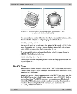
A More Complex Dataset
Create a more complicated volume dataset by performing some trigonometric
operations on the array SPHERE. Add the following line in front of the call to
SHADE_VOLUME:
S = COS(SIN(SPHERE))
This new volume dataset is interesting at the
density value 0.6. To see the iso-surface defined
by the value 0.6, change the call to
SHADE_VOLUME to the line below:
SHADE_VOLUME, S, 0.6, V, P
The SCALE3 and TV commands remain valid.
Save, compile, and execute sphere.pro. You
should see the graphic at the left.](https://image.slidesharecdn.com/idlbasics-190222151049/85/Idl-basics-82-320.jpg)

![basics.bk : animate.doc 84 Mon Apr 28 12:26:12 1997
84 Chapter 12: Animation
Displaying a Series of Images IDL Basics
Displaying a Series of Images
Let’s create an animation that shows a series of images that represent an abnormal
heartbeat. First, read in the images to be displayed. The file abnorm.dat holds
a series of 16 images. Open the file and prepare it for reading by entering the
following commands at the IDL prompt:
OPENR, 1, FILEPATH('abnorm.dat', SUBDIR = ['examples', 'data'])
This command opens the file abnorm.dat for
reading. The FILEPATH command, used as an
argument to OPENR, returns the complete path
to abnorm.dat.
The file holds 16 images of a human heart as 64
by 64 element arrays of bytes, as shown to the
left. Enter the following commands at the IDL
Command Input Line:
H = BYTARR(64, 64, 16) Create a variable to hold the im-
ages.
READU, 1, H Read the images into variable H.
CLOSE, 1 Close the file.
The first command defines H as a 64 by 64 by 16 element array of bytes. The
second uses the unformatted read command to read the images into the variable
H. Load an appropriate color table and display the first image in the array H by
entering:
LOADCT, 3
ERASE
TV, H[*, *, 0]
The asterisks (*) in the first two element positions tell IDL to use all of the
elements in those positions. Hence, the TV command displays a 64 by 64 byte
image. The image is rather small, so resize each image in the array with bilinear
interpolation by entering:
H = REBIN(H, 320, 320, 16)
TV, H[*, *, 0]
Each image in H is 5 times its previous size.](https://image.slidesharecdn.com/idlbasics-190222151049/85/Idl-basics-90-320.jpg)
![basics.bk : animate.doc 85 Mon Apr 28 12:26:12 1997
Chapter 12: Animation 85
IDL Basics Displaying the Animation as a Wire Mesh Surface
Now we can use a simple FOR statement to “animate” the images. (A more robust
and convenient animation routine, XINTERANIMATE, is described below.)
Enter:
FOR, i = 0, 15 DO TVSCL, H[*,*,i]
IDL displays the 16 images in the array H sequentially. To repeat the animation,
press the “up arrow” key to recall the command and press “Return.”
Displaying the Animation as a Wire Mesh Surface
The same series of images can be displayed as different types of animations. For
example, each frame of the animation could be displayed as a SURFACE plot.
Enter the :
S=REBIN(H, 32, 32, 16) Create a new array to hold the
heartbeat data.
S now holds 32 byte by 32 byte versions of the
heartbeat images. SURFACE plots are often
more legible when made from a resized
version of the dataset with fewer data points
in it. Display the first image in S, shown to the
left, as a wire-mesh surface by entering:
SURFACE, S[*,*,0]
Now create a whole series of SURFACE plots,
one for each image in the original dataset. First, create a 3-dimensional array to
hold all of the images by entering:
FRAMES = BYTARR(300, 300, 16)
The variable FRAMES will hold sixteen, 300 by 300 byte images. Now create a 300
by 300 pixel window in which to display the images:
WINDOW, 1, TITLE='IDL Animation', XSIZE=300, YSIZE=300
The next command draws each frame of the animation. A SURFACE plot is
drawn in the window and then the TVRD command is used to read the image
from the plotting window into the FRAMES array. The FOR loop is used to
increment the array indices. The lines below are actually a single IDL command.
The dollar sign ($) works as a continuation character in IDL and the ampersand
(&) allows multiple commands in the same line. Enter:
FOR i = 0, 15 DO BEGIN SURFACE, S[*,*,i], ZRANGE=[0,250] $
& FRAMES[0,0,i] = TVRD() & END](https://image.slidesharecdn.com/idlbasics-190222151049/85/Idl-basics-91-320.jpg)
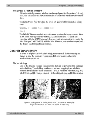
![basics.bk : animate.doc 86 Mon Apr 28 12:26:12 1997
86 Chapter 12: Animation
Animation with XINTERANIMATE IDL Basics
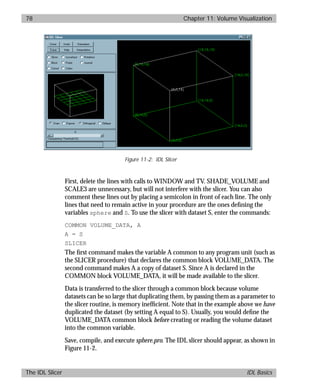
You should see a series of SURFACE plots being drawn in the animation window,
as shown in Figure 12-1. The ZRANGE keyword is used to keep the “height” axis
the same for each plot. Now display the new images in series by entering:
FOR i = 0, 15 DO TV, frames[*,*,i]
Animation with XINTERANIMATE
IDL includes a powerful, widget-based animation tool called
XINTERANIMATE. Sometimes it is useful to view a single wire-mesh surface or
shaded surface from a number of different angles. Let’s make a SURFACE plot
from one of the S dataset frames and view it rotating through 360 degrees. by
entering:
A = S[*,*,0] Save the first frame of the S
datasetinthevariableA tosimpli-
fy the next set of commands.
SURFACE, A, XSTYLE = 4, YSTYLE = 4, ZSTYLE = 4
Display A as a wire-mesh surface.
Setting the XSTYLE, YSTYLE, and ZSTYLE keywords equal to 4 turns axis
drawing off. Usually, IDL automatically scales the axes of plots to best display all
of the data points sent to the plotting routine. However, for this sequence of
images, it is best if each SURFACE plot is drawn with the same size axes. The
SCALE3 procedure can be used to control various aspects of the 3-dimensional
transformation used to display plots. Enter the following:
SCALE3, XRANGE = [0, 31], YRANGE = [0, 31], ZRANGE = [0, 250]
Force the X and Y axis ranges to
run from 0 to 32 and the Z axis
range to run from 0 to 250.
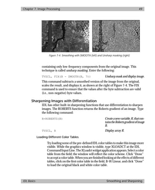
Figure 12-1: SURFACE plots of animation window](https://image.slidesharecdn.com/idlbasics-190222151049/85/Idl-basics-92-320.jpg)
![basics.bk : animate.doc 87 Mon Apr 28 12:26:12 1997
Chapter 12: Animation 87
IDL Basics Clean up the Animation Windows
XINTERANIMATE, SET = [300, 300, 40] Set up the XINTERANIMATE
routinetohold40,300by300byte
images.
FOR i = 0, 39 DO BEGIN SCALE3, AZ = -i * 9 & SURFACE, A, /T3D, $
XST=4, YST=4, ZST=4 & XINTERANIMATE, FRAME=i, WIN=1 & END
Generate each frame of the ani-
mation and store it for the
XINTERANIMATE routine
XINTERANIMATE Play images back as an animation
after all the images have been
saved in the XINTERNIMATE
routine.
The XINTERANIMATE window
should appear, as shown to the left.
“Tape recorder” style controls can be
used to play the animation forward,
play it backward, or stop. Individual
frames can also be selected by moving
the “Animation Frame” slider. The
“Options” menu controls the style and
direction of image playback. Click on
“End Animation” when you are ready
to return to the IDL command line.
Clean up the Animation Windows
Before continuing with the rest of the tutorials, delete the two windows you used
to create the animations. The WDELETE command is used to delete IDL
windows. Delete both window 0 and window 1 by entering:
WDELETE, 0
WDELETE, 1
More Information on Animation with IDL
With just a few IDL commands, you’ve created a number of different types of
animation. For a list of other animation related commands, see the online help
or the IDL HandiGuide quick reference.](https://image.slidesharecdn.com/idlbasics-190222151049/85/Idl-basics-93-320.jpg)

![basics.bk : widgets.doc 92 Mon Apr 28 12:26:12 1997
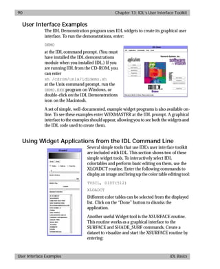
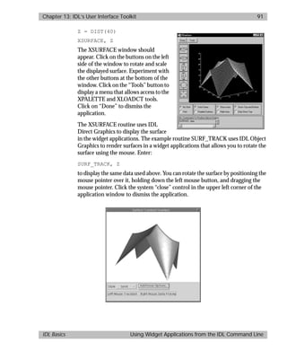
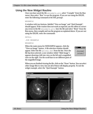
92 Chapter 13: IDL’s User Interface Toolkit
A Sample Widget Application IDL Basics
A Sample Widget Application
The IDL code listed below describes a widget-based application that allows you
to select an image file and display it using a graphical interface. Open an editor
window (or use your own text editor), enter the following lines, and save them in
your current directory with the filename wexample.pro. (If you create your
own routines, you will probably want to create a new subdirectory in which to
store them. When you upgrade to a new version of IDL, the IDL library
subdirectories are updated, so never store your own routines there.) The code for
the routine wexample.pro is shown below:
PRO example_event, event
CASE event.value OF
'Quit Example' : WIDGET_CONTROL, event.top, /DESTROY
'View an Image' : BEGIN
path = FILEPATH('', SUB=['examples', 'data'])
filename = DIALOG_PICKFILE(PATH=path)
IF (STRLEN(filename) EQ 0) THEN RETURN
OPENR, unit, filename, /GET_LUN
fileinfo = FSTAT(unit)
dim = SQRT(fileinfo.size)
image = BYTARR(dim, dim)
READU, unit, image
FREE_LUN, unit
SLIDE_IMAGE, REBIN(image, dim*2, dim*2), $
GROUP = event.top, /REGISTER, RETAIN=2
END
ENDCASE
END
PRO wexample
base = WIDGET_BASE(/COLUMN, XPAD=10, YPAD=10)
menu = CW_BGROUP(base, ['View an Image', 'Quit Example'], $
/COLUMN, /RETURN_NAME)
WIDGET_CONTROL, base, /REALIZE
XMANAGER, 'example', base
END](https://image.slidesharecdn.com/idlbasics-190222151049/85/Idl-basics-98-320.jpg)


![Lab view basics_i[1]](https://cdn.slidesharecdn.com/ss_thumbnails/labviewbasicsi1-110919001249-phpapp01-thumbnail.jpg?width=640&height=640&fit=bounds)