1. Lucene and Juru at Trec 2007: 1-Million Queries Track
Doron Cohen, Einat Amitay, David Carmel
IBM Haifa Research Lab
Haifa 31905, Israel
Email: {doronc,einat,carmel}@il.ibm.com
ABSTRACT
Lucene is an increasingly popular open source search library.
However, our experiments of search quality for TREC data
and evaluations for out-of-the-box Lucene indicated inferior
quality comparing to other systems participating in TREC.
In this work we investigate the differences in measured
search quality between Lucene and Juru, our home-brewed
search engine, and show how Lucene scoring can be modified
to improve its measured search quality for TREC.
Our scoring modifications to Lucene were trained over the
150 topics of the tera-byte tracks. Evaluations of these mod-
ifications with the new - sample based - 1-Million Queries
Track measures - NEU-Map and -Map - indicate the ro-
bustness of the scoring modifications: modified Lucene per-
forms well when compared to stock Lucene and when com-
pared to other systems that participated in the 1-Million
Queries Track this year, both for the training set of 150
queries and for the new measures. As such, this also sup-
ports the robustness of the new measures tested in this track.
This work reports our experiments and results and de-
scribes the modifications involved - namely normalizing term
frequencies, different choice of document length normaliza-
tion, phrase expansion and proximity scoring.
1. INTRODUCTION
Our experiments this year for the TREC 1-Million Queries
Track focused on the scoring function of Lucene, an Apache
open-source search engine [4]. We used our home-brewed
search engine, Juru [2], to compare with Lucene on the 10K
track’s queries over the gov2 collection.
Lucene1
is an open-source library for full-text indexing
and searching in Java. The default scoring function of Lucene
implements the cosine similarity function, while search terms
are weighted by the tf-idf weighting mechanism. Equation 1
describes the default Lucene score for a document d with
respect to a query q:
Score(d, q) =
t∈q
tf(t, d) · idf(t) · (1)
boost(t, d) · norm(d)
where
1
We used Lucene Java: http://lucene.apache.org/java/docs, the first and
main Lucene implementation. Lucene defines a file for-
mat, and so there are ports of Lucene to other languages.
Throughout this work, ”Lucene” refers to ”Apache Lucene
Java”.
• tf(t, d) is the term frequency factor for the term t in
the document d, computed as freq(t, d).
• idf(t) is the inverse document frequency of the term,
computed as 1 + log numDocs
docF req(t)+1
.
• boost(t.field, d) is the boost of the field of t in d, as
set during indexing.
• norm(d) is the normalization value, given the number
of terms within the document.
For more details on Lucene scoring see the official Lucene
scoring2
document.
Our main goal in this work was to experiment with the
scoring mechanism of Lucene in order to bring it to the
same level as the state-of-the-art ranking formulas such as
OKAPI [5] and the SMART scoring model [1]. In order
to study the scoring model of Lucene in full details we ran
Juru and Lucene over the 150 topics of the tera-byte tracks,
and over the 10K queries of the 1-Million Queries Track of
this year. We then modified Lucene’s scoring function to
include better document length normalization, and a better
term-weight setting according to the SMART model. Equa-
tion 2 describes the term frequency (tf) and the normaliza-
tion scheme used by Juru, based on SMART scoring mech-
anism, that we followed to modify Lucene scoring model.
tf(t, d) =
log(1+freq(t,d))
log(1+avg(freq(d)))
(2)
norm(d) = 0.8 avg(#uniqueTerms) + 0.2 #uniqueTerms(d)
As we later describe, we were able to get better results
with a simpler length normalization function that is avail-
able within Lucene, though not as the default length nor-
malization.
For both Juru and Lucene we used the same HTML parser
to extract content of the Web documents of the gov2 collec-
tion. In addition, for both systems the same anchor text ex-
traction process took place. Anchors data was used for two
purposes: 1) Set a document static score according to the
number of in-links pointing to it. 2) Enrich the document
content with the anchor text associated with its in-links.
Last, for both Lucene and Juru we used a similar query
parsing mechanism, which included stop-word removal, syn-
onym expansion and phrase expansion.
2
http://lucene.apache.org/java/2_3_0/scoring.html

2. In the following we describe these processes in full de-
tails and the results both for the 150 topics of the tera-
byte tracks, and for the 10K queries of the 1-Million Queries
Track.
2. ANCHOR TEXT EXTRACTION
Extracting anchor text is a necessary task for indexing
Web collections: adding text surrounding a link to the in-
dexed document representing the linked page. With inverted
indexes it is often inefficient to update a document once it
was indexed. In Lucene, for example, updating an indexed
document involves removing that document from the index
and then (re) adding the updated document. Therefore, an-
chor extraction is done prior to indexing, as a global com-
putation step. Still, for large collections, this is a nontrivial
task. While this is not a new problem, describing a timely
extraction method may be useful for other researchers.
2.1 Extraction method
Our gov2 input is a hierarchical directory structure of
about 27,000 compressed files, each containing multiple doc-
uments (or pages), altogether about 25,000,000 documents.
Our output is a similar directory structure, with one com-
pressed anchors text file for each original pages text file.
Within the file, anchors texts are ordered the same as pages
texts, allowing indexing the entire collection in a single com-
bined scan of the two directories. We now describe the ex-
traction steps.
• (i) Hash by URL: Input pages are parsed, emitting
two types of result lines: page lines and anchor lines.
Result lines are hashed into separate files by URL,
and so for each page, all anchor lines referencing it are
written to the same file as its single page line.
• (ii) Sort lines by URL: This groups together every
page line with all anchors that reference that page.
Note that sort complexity is relative to the files size,
and hence can be controlled by the hash function used.
• (iii) Directory structure: Using the file path info
of page lines, data is saved in new files, creating a
directory structure identical to that of the input.
• (iv) Documents order: Sort each file by document
numbers of page lines. This will allow to index pages
with their anchors.
Note that the extraction speed relies on serial IO in the
splitting steps (i), (iii), and on sorting files that are not too
large in steps (ii), (iv).
2.2 Gov2 Anchors Statistics
Creating the anchors data for gov2 took about 17 hours
on a 2-way Linux. Step (i) above ran in 4 parallel threads
and took most of the time: 11 hours. The total size of the
anchors data is about 2 GB.
We now list some interesting statistics on the anchors
data:
• There are about 220 million anchors for about 25 mil-
lion pages, an average of about 9 anchors per page.
• Maximum number of anchors of a single page is
1,275,245 - that many .gov pages are referencing the
page www.usgs.gov.
• 17% of the pages have no anchors at all.
• 77% of the pages have 1 to 9 anchors.
• 5% of the pages have 10 to 99 anchors.
• 159 pages have more than 100,000 anchors.
Obviously, for pages with many anchors only part of the
anchors data was indexed.
2.3 Static scoring by link information
The links into a page may indicate how authoritative that
page is. We employed a simplistic approach of only count-
ing the number of such in-links, and using that counter to
boost up candidate documents, so that if two candidate
pages agree on all quality measures, the page with more
incoming links would be ranked higher.
Static score (SS) values are linearly combined with textual
scores. Equation 3 shows the static score computation for a
document d linked by in(d) other pages.
SS(d) = min(1,
in(d)
400
) (3)
It is interesting to note that our experiments showed con-
flicting effects of this static scoring: while SS greatly im-
proves Juru’s quality results, SS have no effect with Lucene.
To this moment we do not understand the reason for this
difference of behavior. Therefore, our submissions include
static scoring by in-links count for Juru but not for Lucene.
3. QUERY PARSING
We used a similar query parsing process for both search
engines. The terms extracted from the query include single
query words, stemmed by the Porter stemmer which pass
the stop-word filtering process, lexical affinities, phrases and
synonyms.
3.1 Lexical affinities
Lexical affinities (LAs) represent the correlation between
words co-occurring in a document. LAs are identified by
looking at pairs of words found in close proximity to each
other. It has been described elsewhere [3] how LAs improve
precision of search by disambiguating terms.
During query evaluation, the query profile is constructed
to include the query’s lexical affinities in addition to its in-
dividual terms. This is achieved by identifying all pairs of
words found close to each other in a window of some prede-
fined small size (the sliding window is only defined within
a sentence). For each LA=(t1,t2), Juru creates a pseudo
posting list by finding all documents in which these terms
appear close to each other. This is done by merging the
posting lists of t1 and t2. If such a document is found, it
is added to the posting list of the LA with all the relevant
occurrence information. After creating the posting list, the
new LA is treated by the retrieval algorithm as any other
term in the query profile.
In order to add lexical affinities into Lucene scoring we
used Lucene’s SpanNearQuery which matches spans of the
query terms which are within a given window in the text.

3. 3.2 Phrase expansion
The query is also expanded to include the query text as
a phrase. For example, the query ‘U.S. oil industry history’
is expanded to ‘U.S. oil industry history. ”U.S. oil industry
history” ’. The idea is that documents containing the query
as a phrase should be biased compared to other documents.
The posting list of the query phrase is created by merging
the postings of all terms, considering only documents con-
taining the query terms in adjacent offsets and in the right
order. Similarly to LA weight which specifies the relative
weight between an LA term and simple keyword term, a
phrase weight specifies the relative weight of a phrase term.
Phrases are simulated by Lucene using the PhraseQuery
class.
3.3 Synonym Expansion
The 10K queries for the 1-Million Queries Track track are
strongly related to the .gov domain hence many abbrevia-
tions are found in the query list. For example, the u.s. states
are usually referred by abbreviations (e.g. “ny” for New-
York, “ca” or “cal” for California). However, in many cases
relevant documents refer to the full proper-name rather than
its acronym. Thus, looking only for documents containing
the original query terms will fail to retrieve those relevant
documents.
We therefore used a synonym table for common abbre-
viations in the .gov domain to expand the query. Given a
query term with an existing synonym in the table, expansion
is done by adding the original query phrase while replacing
the original term with its synonym. For example, the query
“ca veterans” is expanded to “ca veterans. California vet-
erans”.
It is however interesting to note that the evaluations of our
Lucene submissions indicated no measurable improvements
due to this synonym expansion.
3.4 Lucene query example
To demonstrate our choice of query parsing, for the origi-
nal topic – ”U.S. oil industry history”, the following Lucene
query was created:
oil industri histori
(
spanNear([oil, industri], 8, false)
spanNear([oil, histori], 8, false)
spanNear([industri, histori], 8, false)
)^4.0
"oil industri histori"~1^0.75
The result Lucene query illustrates some aspects of our
choice of query parsing:
• ”U.S.” is considered a stop word and was removed from
the query text.
• Only stemmed forms of words are used.
• Default query operator is OR.
• Words found in a document up to 7 positions apart
form a lexical affinity. (8 in this example because of
the stopped word.)
• Lexical affinity matches are boosted 4 times more than
single word matches.
• Phrase matches are counted slightly less than single
word matches.
• Phrases allow fuzziness when words were stopped.
For more information see the Lucene query syntax3
doc-
ument.
4. LUCENE SCORE MODIFICATION
Our TREC quality measures for the gov2 collection re-
vealed that the default scoring4
of Lucene is inferior to that
of Juru. (Detailed run results are given in Section 6.)
We were able to improve Lucene’s scoring by changing
the scoring in two areas: document length normalization
and term frequency (tf) normalization.
Lucene’s default length normalization5
is given in equa-
tion 4, where L is the number of words in the document.
lengthNorm(L) =
1
√
L
(4)
The rational behind this formula is to prevent very long
documents from ”taking over” just because they contain
many terms, possibly many times. However a negative side
effect of this normalization is that long documents are ”pun-
ished” too much, while short documents are preferred too
much. The first two modifications below remedy this fur-
ther.
4.1 Sweet Spot Similarity
Here we used the document length normalization of ”Sweet
Spot Similarity”6
. This alternative Similarity function is
available as a Lucene’s ”contrib” package. Its normaliza-
tion value is given in equation 5, where L is the number of
document words.
lengthNorm(L) = (5)
1√
steepness∗(|L−min|+|L−max|−(max−min))+1)
We used steepness = 0.5, min = 1000, and max =
15, 000. This computes to a constant norm for all lengths in
the [min, max] range (the ”sweet spot”), and smaller norm
values for lengths out of this range. Documents shorter or
longer than the sweet spot range are ”punished”.
4.2 Pivoted length normalization
Our pivoted document length normalization follows the
approach of [6], as depicted in equation 6, where U is the
number of unique words in the document and pivot is the
average of U over all documents.
lengthNorm(L) =
1
(1 − slope) ∗ pivot + slope ∗ U
(6)
For Lucene we used slope = 0.16.
3
http://lucene.apache.org/java/2_3_0/queryparsersyntax.html
4
http://lucene.apache.org/java/2_3_0/scoring.html
5
http://lucene.apache.org/java/2_3_0/api/org/apache/lucene/search/DefaultSimilarity.html
6
http://lucene.apache.org/java/2_3_0/api/org/apache/lucene/misc/SweetSpotSimilarity.html

4. 4.3 Term Frequency (tf) normalization
The tf-idf formula used in Lucene computes tf(t in d)
as freq(t, d) where freq(t, d) is the frequency of t in d,
and avgFreq(d) is the average of freq(t, d) over all terms t
of document d. We modified this to take into account the
average term frequency in d, similar to Juru, as shown in
formula 7.
tf(t, d) =
log(1 + freq(t, d))
log(1 + avgFreq(d))
(7)
This distinguishes between terms that highly represent
a document, to terms that are part of duplicated text. In
addition, the logarithmic formula has much smaller variation
than Lucene’s original square root based formula, and hence
the effect of freq(t, d) on the final score is smaller.
4.4 Query fewer fields
Throughout our experiments we saw that splitting the
document text into separate fields, such as title, abstract,
body, anchor, and then (OR) querying all these fields per-
forms poorer than querying a single, combined field. We
have not fully investigated the causes for this, but we suspect
that this too is due to poor length normalization, especially
in the presence of very short fields.
Our recommendation therefore is to refrain from splitting
the document text into fields in those cases that all the fields
are actually searched at the same time.
While splitting into fields allows easy boosting of certain
fields at search time, a better alternative is to boost the
terms themselves, either statically by duplicating them at
indexing time, or perhaps even better dynamically at search
time, e.g. by using term payload values, a new Lucene fea-
ture. In this work we took the first, more static approach.
5. QUERY LOG ANALYSIS
This year’s task resembled a real search environment mainly
because it provided us with a substantial query log. The log
itself provides a glimpse into what it is that users of the
.gov domain actually want to find. This is important since
log analysis has become one of the better ways to improve
search quality and performance.
For example, for our index we created a stopword list from
the most frequent terms appearing in the queries, crossed
with their frequency in the collection. The most obvious
characteristic of the flavor of the queries is the term state
which is ranked as the 6th most frequent query term with
342 mentions, and similarly it is mentioned 10,476,458 times
in the collection. This demonstrates the bias of both the col-
lection and the queries to content pertaining to state affairs.
Also in the queries are over 270 queries containing us, u.s,
usa, or the phrase “united states” and nearly 150 queries
containing the term federal. The fact is that the underlying
assumption in most of the queries in the log is that the re-
quested information describes US government content. This
may sound obvious since it is after all the gov2 collection,
however, it also means that queries that contain the terms
US, federal, and state actually restrict the results much more
than required in a collection dedicated to exactly that con-
tent. So removing those terms from the queries makes much
sense. We experimented with the removal of those terms
and found that the improvement over the test queries is
substantial.
Term Frequency in query log Frequency in index
of 1228 Originally stopped
in 838 Originally stopped
and 653 Originally stopped
for 586 Originally stopped
the 512 Originally stopped
state 342 10476458
to 312 Originally stopped
a 265 Originally stopped
county 233 3957936
california 204 1791416
tax 203 1906788
new 195 4153863
on 194 Originally stopped
department 169 6997021
what 168 1327739
how 143 Originally stopped
federal 143 4953306
health 135 4693981
city 114 2999045
is 114 Originally stopped
national 104 7632976
court 103 2096805
york 103 1804031
school 100 2212112
with 99 Originally stopped
Table 1: Most frequent terms in the query log.
The log information allowed us to stop general terms along
with collection-specific terms such as US, state, United States,
and federal.
Another problem that arose from using such a diverse log
was that we were able to detect over 400 queries which con-
tained abbreviations marked by a dot, such as fed., gov.,
dept., st. and so on. We have also found numbers such
as in street addresses or date of birth that were sometimes
provided in numbers and sometimes in words. Many of the
queries also contained abbreviations for state names which
is the acceptable written form for referring to states in the
US.
For this purpose we prepared a list of synonyms to expand
the queries to contain all the possible forms of the terms.
For example for a query ”Orange County CA” our system
produced two queries ”Orange County CA” and ”Orange
County California” which were submitted as a single query
combined of both strings. Overall we used a list of about
250 such synonyms which consisted of state abbreviations
(e.g. RI, Rhode Island), common federal authorities’ abbre-
viations (e.g. FBI, FDA, etc.), and translation of numbers
to words (e.g. 1, one, 2, two, etc.).
Although we are aware of the many queries in different
languages appearing in the log, mainly in Spanish, we chose
to ignore cross-language techniques and submit them as they
are. Another aspect we did not cover and that could possible
have made a difference is the processing of over 400 queries
that appeared in a wh question format of some sort. We
speculate that analyzing the syntax of those queries could
have made a good filtering mechanism that may have im-
proved our results.

5. 6. RESULTS
Search quality results of our runs for the 1-Million Queries
Track are given in Table 2. For a description of the various
options see Section 4. The top results in each column are
emphasized. The MAP column refer to the 150 terabyte
track queries that were part of the queries pool. We next
analyze these results.
Figure 1: MAP and NEU-Map
Figure 2: -MAP
Figure 3: Precision cut-offs 5, 10, 20
Run 1, the only Juru run, was used as a target. All the
other runs - 2 to 10 - used Lucene.
Runs 1 (Juru) and 9 (Lucene) - marked with ’(*)’ - are the
only runs in this table that were submitted to the 1 Million
Queries Track. Two more Lucene runs were submitted, with
Figure 4: -MAP Recomputed
Figure 5: Search time (seconds/query)
variations of synonym expansion and spell correction, but
their results were nearly identical to Run 9, and these two
runs are therefore not discussed separately in this report.
Also note that Lucene Run 10, which was not submitted,
outperforms the submitted Lucene runs in all measures but
NEU-Map.
Run 2 is the default - out-of-the-box Lucene. This run was
used as a base line for improving Lucene quality measures.
Comparing run 2 with run 1 shows that Lucene’s default
behavior does not perform very well, with MAP of 0.154
comparing to Juru’s MAP of 0.313.
Runs 3, 4, 5 add proximity (LA), phrase, and both prox-
imity and phrase, on top of the default Lucene1. The results
for Run 5 reveals that adding both proximity and phrase to
the query evaluation is beneficial, and we therefore pick this
configuration as the base for the rest of the evaluation, and
name it as Lucene4. Note then that runs 6 to 9 are marked
as Lucene4 as well, indicating proximity and phrase in all of
them.
Lucene’s sweet spot similarity run performs much better
than the default Lucene behavior, bringing MAP from 0.214
in run 5 to 0.273 in run 7. Note that the only change here
is a different document length normalization. Replacing the
document length normalization with a pivoted length one in
run 6 improves MAP further to 0.284.
Run 10 is definitely the best run: combining the docu-
ment length normalization of Lucene’s sweet spot similarity
with normalizing the tf by the average term frequency in a
document. This combination brings Lucene’s MAP to 0.306,
and even outperforms Juru for the P@5, P@10, and P@20

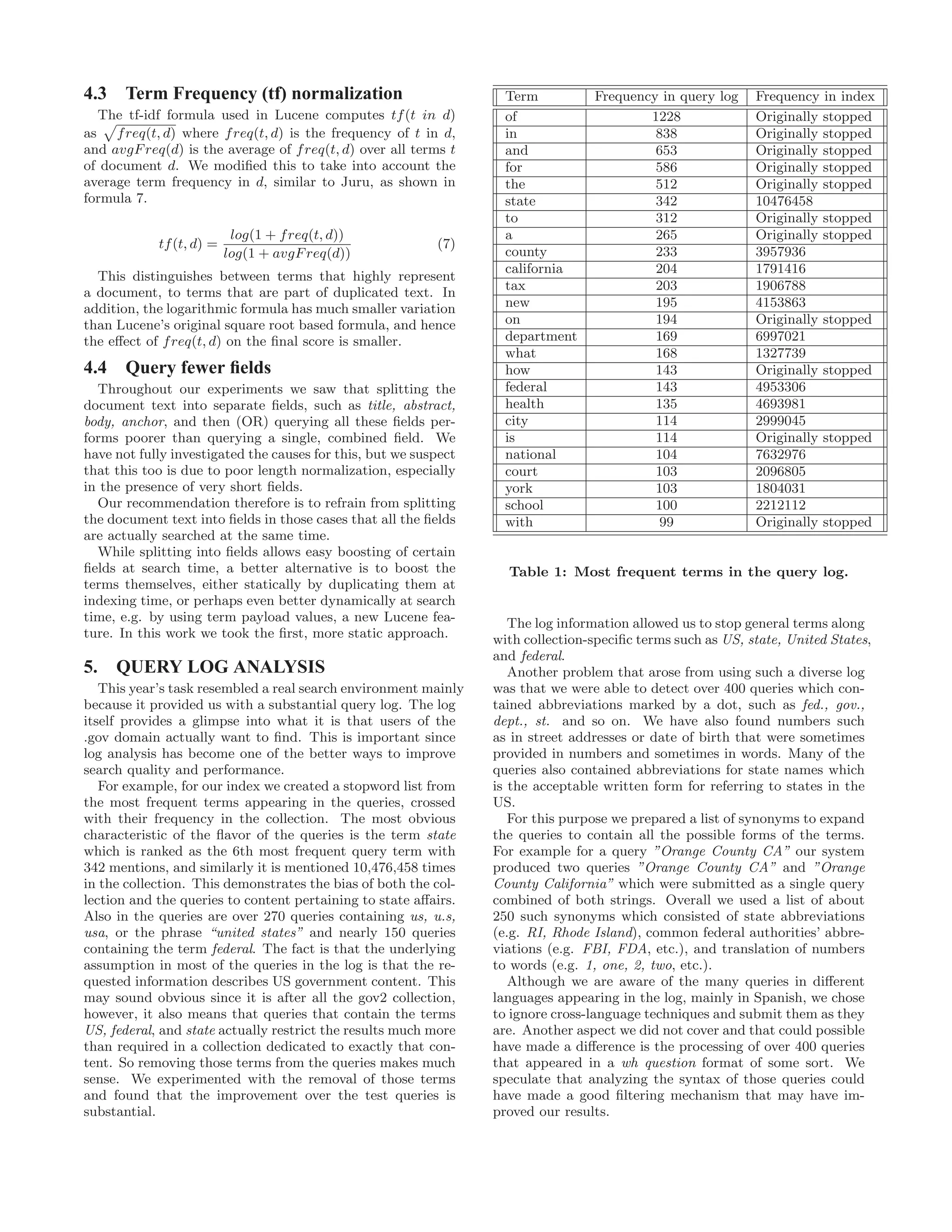
6. Run MAP -Map NEU-Map P@5 P@10 P@20
-Map
sec/q
Recomputed
1. Juru (*) 0.313 0.1080 0.3199 0.592 0.560 0.529 0.2121
2. Lucene1 Base 0.154 0.0746 0.1809 0.313 0.303 0.289 0.0848 1.4
3. Lucene2 LA 0.208 0.0836 0.2247 0.409 0.382 0.368 0.1159 5.6
4. Lucene3 Phrase 0.191 0.0789 0.2018 0.358 0.347 0.341 0.1008 4.1
5. Lucene4 LA + Phrase 0.214 0.0846 0.2286 0.409 0.390 0.383 0.1193 6.7
6. Lucene4 Pivot Length Norm 0.284 0.572 0.540 0.503
7. Lucene4 Sweet Spot Similarity 0.273 0.1059 0.2553 0.593 0.565 0.527 0.1634 6.9
8. Lucene4 TF avg norm 0.194 0.0817 0.2116 0.404 0.373 0.370 0.1101 7.8
9. Lucene4 Pivot + TF avg norm (*) 0.294 0.1031 0.3255 0.587 0.542 0.512 0.1904
10. Lucene4 Sweet Spot + TF avg norm 0.306 0.1091 0.3171 0.627 0.589 0.543 0.2004 8.0
Table 2: Search Quality Comparison.
measures.
The 1-Million Queries Track measures of -Map and NEU-
Map introduced in the 1-Million Queries Track support the
improvements to Lucene scoring: runs 9 and 10 are the best
Lucene runs in these measures as well, with a slight dis-
agreement in the NEU-Map measure that prefers run 9.
Figures 1 and 2 show that the improvements of stock
Lucene are consistent for all three measures: MAP, -Map
and NEU-Map. Figure 3 demonstrates similar consistency
for precision cut-offs at 5, 10 and 20.
Since most of the runs analyzed here were not submitted,
we applied the supplied expert utility to generated a new
expert.rels file, using all our runs. As result, the evaluate
program that computes -Map was able to take into account
any new documents retrieved by the new runs, however, this
ignored any information provided by any other run. Note:
it is not that new unjudged documents were treated as rele-
vant, but the probabilities that a non-judged document re-
trieved by the new runs is relevant were computed more
accurately this way.
Column -Map2 in Table 2 show this re-computation of
-Map, and, together with Figure 4, we can see that the
improvements to Lucene search quality are consistent with
previous results, and run 10 is the best Lucene run.
Finally, we measured the search time penalty for the qual-
ity improvements. This is depicted in column sec/q of Table
2 as well as Figure 5. We can see that the search time grew
by a factor of almost 6. This is a significant cost, that surely
some applications would not be able to afford. However it
should be noticed that in this work we focused on search
quality and so better search time is left for future work.
7. SUMMARY
We started by measuring Lucene’s out of the box search
quality for TREC data and found that it is significantly
inferior to other search engines that participate in TREC,
and in particular comparing to our search engine Juru.
We were able to improve Lucene’s search quality as mea-
sured for TREC data by (1) adding phrase expansion and
proximity scoring to the query, (2) better choice of docu-
ment length normalization, and (3) normalizing tf values by
document’s average term frequency. We also would like to
note the high performance of improved Lucene over the new
query set – Lucene three submitted runs were ranked first
according to the NEU measure and in places 2-4 (after the
Juru run) according to eMap.
The improvements that were trained on the 150 terabyte
queries of previous years were shown consistent with the
1755 judged queries of the 1-Million Queries Track, and with
the new sampling measures -Map and NEU-Map.
Application developers using Lucene can easily adopt the
document length normalization part of our work, simply by
a different similarity choice. Phrase expansion of the query
as well as proximity scoring should be also relatively easy
to add. However for applying the tf normalization some
changes in Lucene code would be required.
Additional considerations that search application devel-
opers should take into account are the search time cost, and
whether the improvements demonstrated here are also rele-
vant for the domain of the specific search application.
8. ACKNOWLEDGMENTS
We would like to thank Ian Soboroff and Ben Carterette
for sharing their insights in discussions about how the results
- all the results and ours - can be interpreted for the writing
of this report.
Also thanks to Nadav Har’El for helpful discussions on
anchor text extraction, and for his code to add proximity
scoring to Lucene.
9. REFERENCES
[1] C. Buckley, A. Singhal, and M. Mitra. New retrieval
approaches using smart: Trec 4. In TREC, 1995.
[2] D. Carmel and E. Amitay. Juru at TREC 2006: TAAT
versus DAAT in the Terabyte Track. In Proceedings of
the 15th Text REtrieval Conference (TREC2006).
National Institute of Standards and Technology. NIST,
2006.
[3] D. Carmel, E. Amitay, M. Herscovici, Y. S. Maarek,
Y. Petruschka, and A. Soffer. Juru at TREC 10 -
Experiments with Index Pruning. In Proceeding of
Tenth Text REtrieval Conference (TREC-10). National
Institute of Standards and Technology. NIST, 2001.
[4] O. Gospodnetic and E. Hatcher. Lucene in Action.
Manning Publications Co., 2005.
[5] S. E. Robertson, S. Walker, M. Hancock-Beaulieu,
M. Gatford, and A. Payne. Okapi at trec-4. In TREC,
1995.
[6] A. Singhal, C. Buckley, and M. Mitra. Pivoted
document length normalization. In Proceedings of the

7. 19th annual international ACM SIGIR conference on
Research and development in information retrieval,
pages 21–29, 1996.