4 - 2
Outline
▶Global Company Profile:
Walt Disney Parks & Resorts
▶ What Is Forecasting?
▶ The Strategic Importance of
Forecasting
▶ Seven Steps in the Forecasting
System
▶ Forecasting Approaches
3.
4 - 3
Outline- Continued
▶ Time-Series Forecasting
▶ Associative Forecasting Methods:
Regression and Correlation Analysis
▶ Monitoring and Controlling Forecasts
▶ Forecasting in the Service Sector
4.
4 - 4
LearningObjectives
When you complete this chapter you
should be able to :
1. Understand the three time horizons and
which models apply for each use
2. Explain when to use each of the four
qualitative models
3. Apply the naive, moving average,
exponential smoothing, and trend
methods
5.
4 - 5
LearningObjectives
When you complete this chapter you
should be able to :
4. Compute three measures of forecast
accuracy
5. Develop seasonal indices
6. Conduct a regression and correlation
analysis
7. Use a tracking signal
6.
4 - 6
►Global portfolio includes parks in Hong Kong,
Paris, Tokyo, Orlando, and Anaheim
► Revenues are derived from people – how
many visitors and how they spend their
money
► Daily management report contains only the
forecast and actual attendance at each park
Forecasting Provides a
Competitive Advantage for Disney
7.
4 - 7
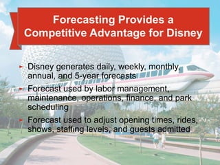
►Disney generates daily, weekly, monthly,
annual, and 5-year forecasts
► Forecast used by labor management,
maintenance, operations, finance, and park
scheduling
► Forecast used to adjust opening times, rides,
shows, staffing levels, and guests admitted
Forecasting Provides a
Competitive Advantage for Disney
8.
4 - 8
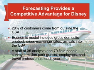
►20% of customers come from outside the
USA
► Economic model includes gross domestic
product, cross-exchange rates, arrivals into
the USA
► A staff of 35 analysts and 70 field people
survey 1 million park guests, employees, and
travel professionals each year
Forecasting Provides a
Competitive Advantage for Disney
9.
4 - 9
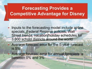
►Inputs to the forecasting model include airline
specials, Federal Reserve policies, Wall
Street trends, vacation/holiday schedules for
3,000 school districts around the world
► Average forecast error for the 5-year forecast
is 5%
► Average forecast error for annual forecasts is
between 0% and 3%
Forecasting Provides a
Competitive Advantage for Disney
10.
4 - 10
Whatis Forecasting?
► Process of predicting a
future event
► Underlying basis
of all business
decisions
► Production
► Inventory
► Personnel
► Facilities
??
11.
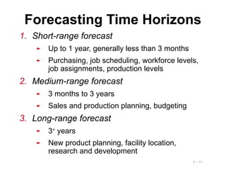
4 - 11
1.Short-range forecast
► Up to 1 year, generally less than 3 months
► Purchasing, job scheduling, workforce levels,
job assignments, production levels
2. Medium-range forecast
► 3 months to 3 years
► Sales and production planning, budgeting
3. Long-range forecast
► 3+
years
► New product planning, facility location,
research and development
Forecasting Time Horizons
12.
4 - 12
DistinguishingDifferences
1. Medium/long range forecasts deal with more
comprehensive issues and support
management decisions regarding planning
and products, plants and processes
2. Short-term forecasting usually employs
different methodologies than longer-term
forecasting
3. Short-term forecasts tend to be more
accurate than longer-term forecasts
13.
4 - 13
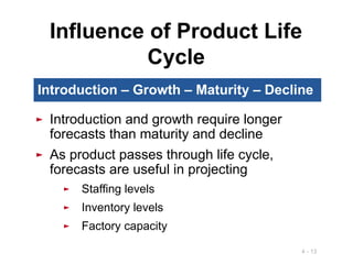
Influenceof Product Life
Cycle
► Introduction and growth require longer
forecasts than maturity and decline
► As product passes through life cycle,
forecasts are useful in projecting
► Staffing levels
► Inventory levels
► Factory capacity
Introduction – Growth – Maturity – Decline
14.
4 - 14
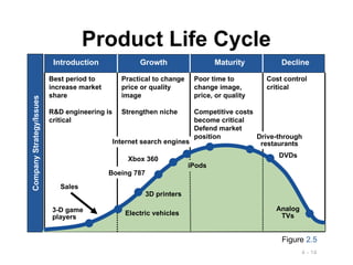
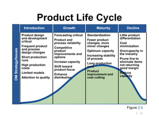
ProductLife Cycle
Best period to
increase market
share
R&D engineering is
critical
Practical to change
price or quality
image
Strengthen niche
Poor time to
change image,
price, or quality
Competitive costs
become critical
Defend market
position
Cost control
critical
Introduction Growth Maturity Decline
Company
Strategy/Issues
Figure 2.5
Internet search engines
Sales
Drive-through
restaurants
DVDs
Analog
TVs
Boeing 787
Electric vehicles
iPods
3-D game
players
3D printers
Xbox 360
15.
4 - 15
ProductLife Cycle
Product design
and development
critical
Frequent product
and process
design changes
Short production
runs
High production
costs
Limited models
Attention to quality
Introduction Growth Maturity Decline
OM
Strategy/Issues
Forecasting critical
Product and
process reliability
Competitive
product
improvements and
options
Increase capacity
Shift toward
product focus
Enhance
distribution
Standardization
Fewer product
changes, more
minor changes
Optimum capacity
Increasing stability
of process
Long production
runs
Product
improvement and
cost cutting
Little product
differentiation
Cost
minimization
Overcapacity in
the industry
Prune line to
eliminate items
not returning
good margin
Reduce
capacity
Figure 2.5
16.
4 - 16
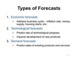
Typesof Forecasts
1. Economic forecasts
► Address business cycle – inflation rate, money
supply, housing starts, etc.
2. Technological forecasts
► Predict rate of technological progress
► Impacts development of new products
3. Demand forecasts
► Predict sales of existing products and services
17.
4 - 17
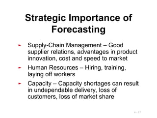
StrategicImportance of
Forecasting
► Supply-Chain Management – Good
supplier relations, advantages in product
innovation, cost and speed to market
► Human Resources – Hiring, training,
laying off workers
► Capacity – Capacity shortages can result
in undependable delivery, loss of
customers, loss of market share
18.
4 - 18
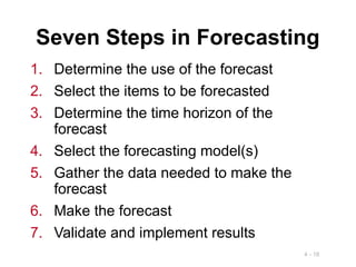
SevenSteps in Forecasting
1. Determine the use of the forecast
2. Select the items to be forecasted
3. Determine the time horizon of the
forecast
4. Select the forecasting model(s)
5. Gather the data needed to make the
forecast
6. Make the forecast
7. Validate and implement results
19.
4 - 19
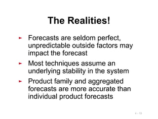
TheRealities!
► Forecasts are seldom perfect,
unpredictable outside factors may
impact the forecast
► Most techniques assume an
underlying stability in the system
► Product family and aggregated
forecasts are more accurate than
individual product forecasts
20.
4 - 20
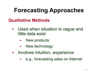
ForecastingApproaches
► Used when situation is vague and
little data exist
► New products
► New technology
► Involves intuition, experience
► e.g., forecasting sales on Internet
Qualitative Methods
21.
4 - 21
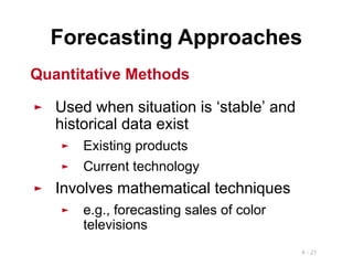
ForecastingApproaches
► Used when situation is ‘stable’ and
historical data exist
► Existing products
► Current technology
► Involves mathematical techniques
► e.g., forecasting sales of color
televisions
Quantitative Methods
22.
4 - 22
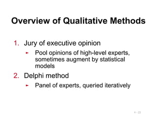
Overviewof Qualitative Methods
1. Jury of executive opinion
► Pool opinions of high-level experts,
sometimes augment by statistical
models
2. Delphi method
► Panel of experts, queried iteratively
23.
4 - 23
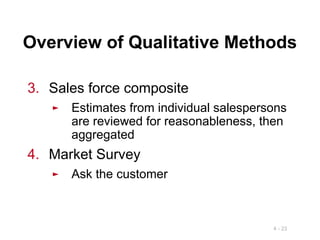
Overviewof Qualitative Methods
3. Sales force composite
► Estimates from individual salespersons
are reviewed for reasonableness, then
aggregated
4. Market Survey
► Ask the customer
24.
4 - 24
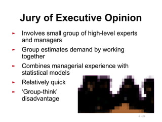
►Involves small group of high-level experts
and managers
► Group estimates demand by working
together
► Combines managerial experience with
statistical models
► Relatively quick
► ‘Group-think’
disadvantage
Jury of Executive Opinion
25.
4 - 25
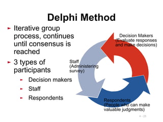
DelphiMethod
► Iterative group
process, continues
until consensus is
reached
► 3 types of
participants
► Decision makers
► Staff
► Respondents
Staff
(Administering
survey)
Decision Makers
(Evaluate responses
and make decisions)
Respondents
(People who can make
valuable judgments)
26.
4 - 26
SalesForce Composite
► Each salesperson projects his or her
sales
► Combined at district and national
levels
► Sales reps know customers’ wants
► May be overly optimistic
27.
4 - 27
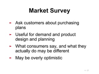
MarketSurvey
► Ask customers about purchasing
plans
► Useful for demand and product
design and planning
► What consumers say, and what they
actually do may be different
► May be overly optimistic
4 - 29
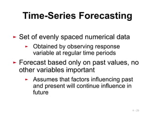
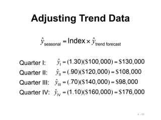
►Set of evenly spaced numerical data
► Obtained by observing response
variable at regular time periods
► Forecast based only on past values, no
other variables important
► Assumes that factors influencing past
and present will continue influence in
future
Time-Series Forecasting
4 - 31
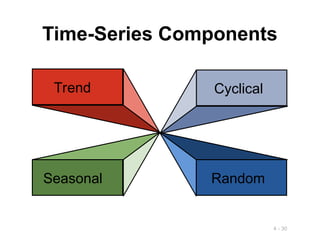
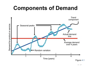
Componentsof Demand
Demand
for
product
or
service
| | | |
1 2 3 4
Time (years)
Average demand
over 4 years
Trend
component
Actual demand
line
Random variation
Figure 4.1
Seasonal peaks
32.
4 - 32
►Persistent, overall upward or
downward pattern
► Changes due to population,
technology, age, culture, etc.
► Typically several years duration
Trend Component
33.
4 - 33
►Regular pattern of up and down
fluctuations
► Due to weather, customs, etc.
► Occurs within a single year
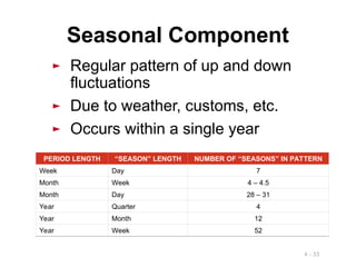
Seasonal Component
PERIOD LENGTH “SEASON” LENGTH NUMBER OF “SEASONS” IN PATTERN
Week Day 7
Month Week 4 – 4.5
Month Day 28 – 31
Year Quarter 4
Year Month 12
Year Week 52
34.
4 - 34
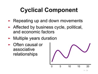
►Repeating up and down movements
► Affected by business cycle, political,
and economic factors
► Multiple years duration
► Often causal or
associative
relationships
Cyclical Component
0 5 10 15 20
35.
4 - 35
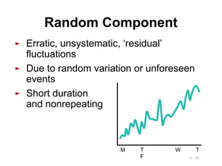
►Erratic, unsystematic, ‘residual’
fluctuations
► Due to random variation or unforeseen
events
► Short duration
and nonrepeating
Random Component
M T W T
F
36.
4 - 36
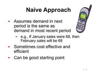
NaiveApproach
► Assumes demand in next
period is the same as
demand in most recent period
► e.g., If January sales were 68, then
February sales will be 68
► Sometimes cost effective and
efficient
► Can be good starting point
37.
4 - 37
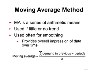
►MA is a series of arithmetic means
► Used if little or no trend
► Used often for smoothing
► Provides overall impression of data
over time
Moving Average Method
38.
4 - 38
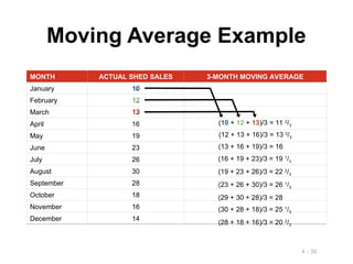
MovingAverage Example
MONTH ACTUAL SHED SALES 3-MONTH MOVING AVERAGE
January 10
February 12
March 13
April 16
May 19
June 23
July 26
August 30
September 28
October 18
November 16
December 14
(10 + 12 + 13)/3 = 11 2
/3
(12 + 13 + 16)/3 = 13 2
/3
(13 + 16 + 19)/3 = 16
(16 + 19 + 23)/3 = 19 1
/3
(19 + 23 + 26)/3 = 22 2
/3
(23 + 26 + 30)/3 = 26 1
/3
(29 + 30 + 28)/3 = 28
(30 + 28 + 18)/3 = 25 1
/3
(28 + 18 + 16)/3 = 20 2
/3
10
12
13
39.
4 - 39
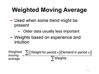
►Used when some trend might be
present
► Older data usually less important
► Weights based on experience and
intuition
Weighted Moving Average
Weighted
moving
average
40.
4 - 40
WeightedMoving Average
MONTH ACTUAL SHED SALES 3-MONTH WEIGHTED MOVING AVERAGE
January 10
February 12
March 13
April 16
May 19
June 23
July 26
August 30
September 28
October 18
November 16
December 14
WEIGHTS APPLIED PERIOD
3 Last month
2 Two months ago
1 Three months ago
6 Sum of the weights
Forecast for this month =
3 x Sales last mo. + 2 x Sales 2 mos. ago + 1 x Sales 3 mos. ago
Sum of the weights
[(3 x 13) + (2 x 12) + (10)]/6 = 12 1
/6
10
12
13
41.
4 - 41
WeightedMoving Average
MONTH ACTUAL SHED SALES 3-MONTH WEIGHTED MOVING AVERAGE
January 10
February 12
March 13
April 16
May 19
June 23
July 26
August 30
September 28
October 18
November 16
December 14
[(3 x 13) + (2 x 12) + (10)]/6 = 12 1
/6
10
12
13
[(3 x 16) + (2 x 13) + (12)]/6 = 14 1
/3
[(3 x 19) + (2 x 16) + (13)]/6 = 17
[(3 x 23) + (2 x 19) + (16)]/6 = 20 1
/2
[(3 x 26) + (2 x 23) + (19)]/6 = 23 5
/6
[(3 x 30) + (2 x 26) + (23)]/6 = 27 1
/2
[(3 x 28) + (2 x 30) + (26)]/6 = 28 1
/3
[(3 x 18) + (2 x 28) + (30)]/6 = 23 1
/3
[(3 x 16) + (2 x 18) + (28)]/6 = 18 2
/3
42.
4 - 42
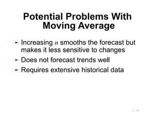
►Increasing n smooths the forecast but
makes it less sensitive to changes
► Does not forecast trends well
► Requires extensive historical data
Potential Problems With
Moving Average
43.
4 - 43
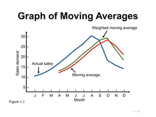
Graphof Moving Averages
| | | | | | | | | | | |
J F M A M J J A S O N D
Sales
demand
30 –
25 –
20 –
15 –
10 –
5 –
Month
Actual sales
Moving average
Weighted moving average
Figure 4.2
44.
4 - 44
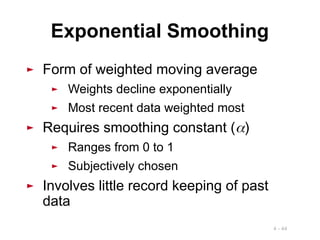
►Form of weighted moving average
► Weights decline exponentially
► Most recent data weighted most
► Requires smoothing constant ()
► Ranges from 0 to 1
► Subjectively chosen
► Involves little record keeping of past
data
Exponential Smoothing
45.
4 - 45
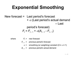
ExponentialSmoothing
New forecast = Last period’s forecast
+ (Last period’s actual demand
– Last
period’s forecast)
Ft = Ft – 1 + (At – 1 - Ft – 1)
where Ft = new forecast
Ft – 1 = previous period’s forecast
= smoothing (or weighting) constant (0 ≤ ≤ 1)
At – 1 = previous period’s actual demand
46.
4 - 46
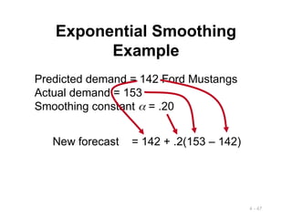
ExponentialSmoothing
Example
Predicted demand = 142 Ford Mustangs
Actual demand = 153
Smoothing constant = .20
47.
4 - 47
ExponentialSmoothing
Example
Predicted demand = 142 Ford Mustangs
Actual demand = 153
Smoothing constant = .20
New forecast = 142 + .2(153 – 142)
48.
4 - 48
ExponentialSmoothing
Example
Predicted demand = 142 Ford Mustangs
Actual demand = 153
Smoothing constant = .20
New forecast = 142 + .2(153 – 142)
= 142 + 2.2
= 144.2 ≈ 144 cars
49.
4 - 49
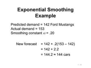
Effectof
Smoothing Constants
▶ Smoothing constant generally .05 ≤ ≤ .50
▶ As increases, older values become less
significant
WEIGHT ASSIGNED TO
SMOOTHING
CONSTANT
MOST
RECENT
PERIOD
()
2ND
MOST
RECENT
PERIOD
(1 – )
3RD
MOST
RECENT
PERIOD
(1 – )2
4th
MOST
RECENT
PERIOD
(1 – )3
5th
MOST
RECENT
PERIOD
(1 – )4
= .1 .1 .09 .081 .073 .066
= .5 .5 .25 .125 .063 .031
4 - 51
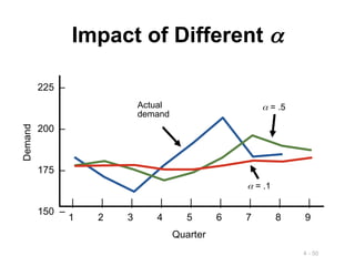
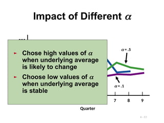
Impactof Different
225 –
200 –
175 –
150 –
| | | | | | | | |
1 2 3 4 5 6 7 8 9
Quarter
Demand
= .1
Actual
demand
= .5
► Chose high values of
when underlying average
is likely to change
► Choose low values of
when underlying average
is stable
52.
4 - 52
Choosing
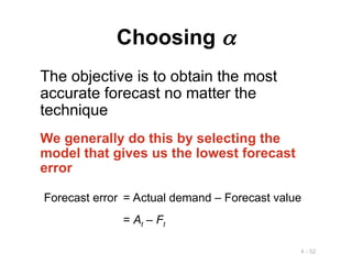
The objective is to obtain the most
accurate forecast no matter the
technique
We generally do this by selecting the
model that gives us the lowest forecast
error
Forecast error = Actual demand – Forecast value
= At – Ft
53.
4 - 53
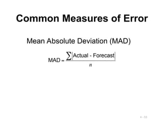
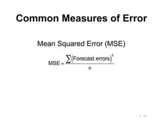
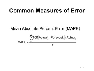
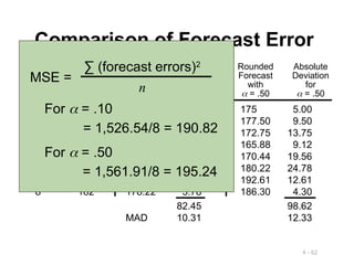
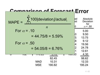
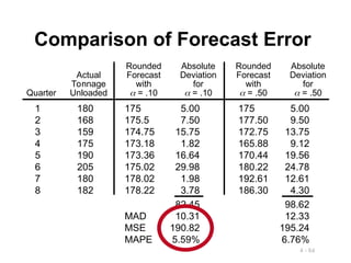
CommonMeasures of Error
Mean Absolute Deviation (MAD)
4 - 73
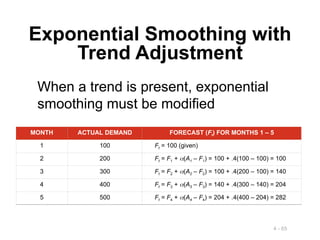
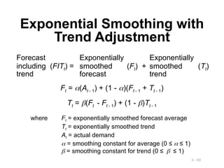
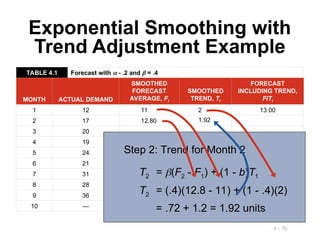
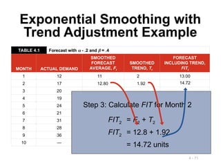
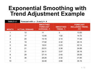
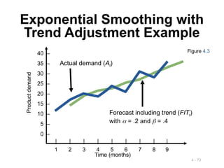
ExponentialSmoothing with
Trend Adjustment Example
Figure 4.3
| | | | | | | | |
1 2 3 4 5 6 7 8 9
Time (months)
Product
demand
40 –
35 –
30 –
25 –
20 –
15 –
10 –
5 –
0 –
Actual demand (At)
Forecast including trend (FITt)
with = .2 and = .4
74.
4 - 74
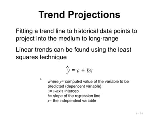
TrendProjections
Fitting a trend line to historical data points to
project into the medium to long-range
Linear trends can be found using the least
squares technique
y = a + bx
^
where y= computed value of the variable to be
predicted (dependent variable)
a= y-axis intercept
b= slope of the regression line
x= the independent variable
^
75.
4 - 75
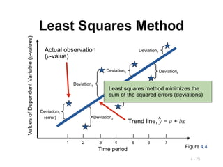
LeastSquares Method
Figure 4.4
Deviation1
(error)
Deviation5
Deviation7
Deviation2
Deviation6
Deviation4
Deviation3
Actual observation
(y-value)
Trend line, y = a + bx
^
Time period
Values
of
Dependent
Variable
(y-values)
| | | | | | |
1 2 3 4 5 6 7
Least squares method minimizes the
sum of the squared errors (deviations)
76.
4 - 76
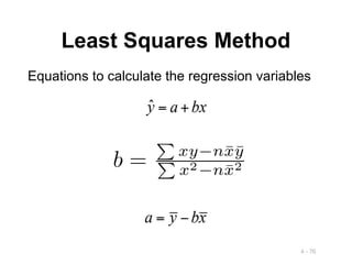
LeastSquares Method
Equations to calculate the regression variables
77.
4 - 77
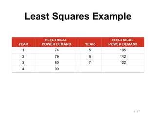
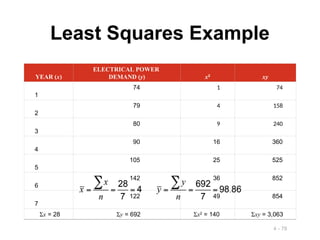
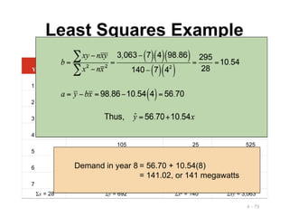
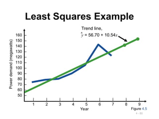
LeastSquares Example
YEAR
ELECTRICAL
POWER DEMAND YEAR
ELECTRICAL
POWER DEMAND
1 74 5 105
2 79 6 142
3 80 7 122
4 90
4 - 81
LeastSquares Requirements
1. We always plot the data to insure a
linear relationship
2. We do not predict time periods far
beyond the database
3. Deviations around the least squares
line are assumed to be random
82.
4 - 82
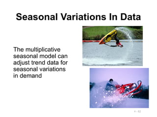
SeasonalVariations In Data
The multiplicative
seasonal model can
adjust trend data for
seasonal variations
in demand
83.
4 - 83
SeasonalVariations In Data
1. Find average historical demand for each month
2. Compute the average demand over all months
3. Compute a seasonal index for each month
4. Estimate next year’s total demand
5. Divide this estimate of total demand by the
number of months, then multiply it by the
seasonal index for that month
Steps in the process for monthly seasons:
84.
4 - 84
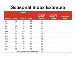
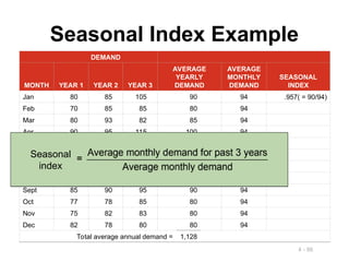
SeasonalIndex Example
DEMAND
MONTH YEAR 1 YEAR 2 YEAR 3
AVERAGE
YEARLY
DEMAND
AVERAGE
MONTHLY
DEMAND
SEASONAL
INDEX
Jan 80 85 105
Feb 70 85 85
Mar 80 93 82
Apr 90 95 115
May 113 125 131
June 110 115 120
July 100 102 113
Aug 88 102 110
Sept 85 90 95
Oct 77 78 85
Nov 75 82 83
Dec 82 78 80
90
80
85
100
123
115
105
100
90
80
80
80
Total average annual demand = 1,128
85.
4 - 85
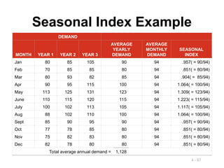
SeasonalIndex Example
DEMAND
MONTH YEAR 1 YEAR 2 YEAR 3
AVERAGE
YEARLY
DEMAND
AVERAGE
MONTHLY
DEMAND
SEASONAL
INDEX
Jan 80 85 105 90 94
Feb 70 85 85 80 94
Mar 80 93 82 85 94
Apr 90 95 115 100 94
May 113 125 131 123 94
June 110 115 120 115 94
July 100 102 113 105 94
Aug 88 102 110 100 94
Sept 85 90 95 90 94
Oct 77 78 85 80 94
Nov 75 82 83 80 94
Dec 82 78 80 80 94
Total average annual demand = 1,128
Average
monthly
demand
86.
4 - 86
SeasonalIndex Example
DEMAND
MONTH YEAR 1 YEAR 2 YEAR 3
AVERAGE
YEARLY
DEMAND
AVERAGE
MONTHLY
DEMAND
SEASONAL
INDEX
Jan 80 85 105 90 94
Feb 70 85 85 80 94
Mar 80 93 82 85 94
Apr 90 95 115 100 94
May 113 125 131 123 94
June 110 115 120 115 94
July 100 102 113 105 94
Aug 88 102 110 100 94
Sept 85 90 95 90 94
Oct 77 78 85 80 94
Nov 75 82 83 80 94
Dec 82 78 80 80 94
Total average annual demand = 1,128
Seasonal
index
.957( = 90/94)
87.
4 - 87
SeasonalIndex Example
DEMAND
MONTH YEAR 1 YEAR 2 YEAR 3
AVERAGE
YEARLY
DEMAND
AVERAGE
MONTHLY
DEMAND
SEASONAL
INDEX
Jan 80 85 105 90 94 .957( = 90/94)
Feb 70 85 85 80 94 .851( = 80/94)
Mar 80 93 82 85 94 .904( = 85/94)
Apr 90 95 115 100 94 1.064( = 100/94)
May 113 125 131 123 94 1.309( = 123/94)
June 110 115 120 115 94 1.223( = 115/94)
July 100 102 113 105 94 1.117( = 105/94)
Aug 88 102 110 100 94 1.064( = 100/94)
Sept 85 90 95 90 94 .957( = 90/94)
Oct 77 78 85 80 94 .851( = 80/94)
Nov 75 82 83 80 94 .851( = 80/94)
Dec 82 78 80 80 94 .851( = 80/94)
Total average annual demand = 1,128
88.
4 - 88
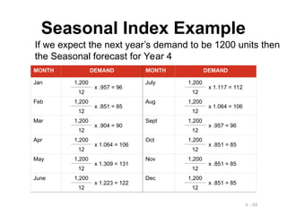
SeasonalIndex Example
MONTH DEMAND MONTH DEMAND
Jan 1,200
x .957 = 96
July 1,200
x 1.117 = 112
12 12
Feb 1,200
x .851 = 85
Aug 1,200
x 1.064 = 106
12 12
Mar 1,200
x .904 = 90
Sept 1,200
x .957 = 96
12 12
Apr 1,200
x 1.064 = 106
Oct 1,200
x .851 = 85
12 12
May 1,200
x 1.309 = 131
Nov 1,200
x .851 = 85
12 12
June 1,200
x 1.223 = 122
Dec 1,200
x .851 = 85
12 12
If we expect the next year’s demand to be 1200 units then
the Seasonal forecast for Year 4
89.
4 - 89
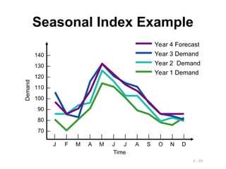
SeasonalIndex Example
140 –
130 –
120 –
110 –
100 –
90 –
80 –
70 –
| | | | | | | | | | | |
J F M A M J J A S O N D
Time
Demand
Year 4 Forecast
Year 3 Demand
Year 2 Demand
Year 1 Demand
90.
4 - 90
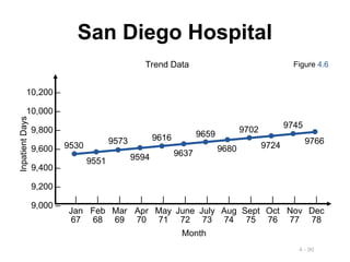
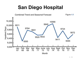
SanDiego Hospital
10,200 –
10,000 –
9,800 –
9,600 –
9,400 –
9,200 –
9,000 –
| | | | | | | | | | | |
Jan Feb Mar Apr May June July Aug Sept Oct Nov Dec
67 68 69 70 71 72 73 74 75 76 77 78
Month
Inpatient
Days
9530
9551
9573
9594
9616
9637
9659
9680
9702
9724
9745
9766
Figure 4.6
Trend Data
91.
4 - 91
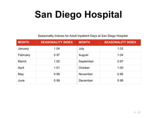
SanDiego Hospital
Seasonality Indices for Adult Inpatient Days at San Diego Hospital
MONTH SEASONALITY INDEX MONTH SEASONALITY INDEX
January 1.04 July 1.03
February 0.97 August 1.04
March 1.02 September 0.97
April 1.01 October 1.00
May 0.99 November 0.96
June 0.99 December 0.98
92.
4 - 92
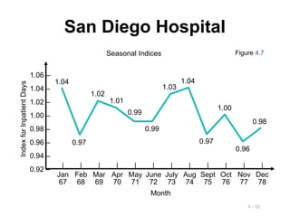
SanDiego Hospital
1.06 –
1.04 –
1.02 –
1.00 –
0.98 –
0.96 –
0.94 –
0.92 –
| | | | | | | | | | | |
Jan Feb Mar Apr May June July Aug Sept Oct Nov Dec
67 68 69 70 71 72 73 74 75 76 77 78
Month
Index
for
Inpatient
Days
1.04
1.02
1.01
0.99
1.03
1.04
1.00
0.98
0.97
0.99
0.97
0.96
Figure 4.7
Seasonal Indices
93.
4 - 93
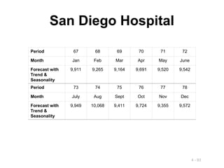
SanDiego Hospital
Period 67 68 69 70 71 72
Month Jan Feb Mar Apr May June
Forecast with
Trend &
Seasonality
9,911 9,265 9,164 9,691 9,520 9,542
Period 73 74 75 76 77 78
Month July Aug Sept Oct Nov Dec
Forecast with
Trend &
Seasonality
9,949 10,068 9,411 9,724 9,355 9,572
94.
4 - 94
SanDiego Hospital
10,200 –
10,000 –
9,800 –
9,600 –
9,400 –
9,200 –
9,000 –
| | | | | | | | | | | |
Jan Feb Mar Apr May June July Aug Sept Oct Nov Dec
67 68 69 70 71 72 73 74 75 76 77 78
Month
Inpatient
Days
Figure 4.8
9911
9265
9764
9520
9691
9411
9949
9724
9542
9355
10068
9572
Combined Trend and Seasonal Forecast
4 - 96
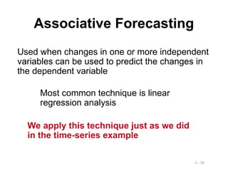
AssociativeForecasting
Used when changes in one or more independent
variables can be used to predict the changes in
the dependent variable
Most common technique is linear
regression analysis
We apply this technique just as we did
in the time-series example
97.
4 - 97
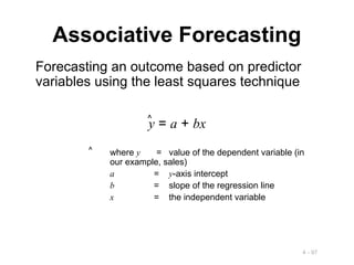
AssociativeForecasting
Forecasting an outcome based on predictor
variables using the least squares technique
y = a + bx
^
where y = value of the dependent variable (in
our example, sales)
a = y-axis intercept
b = slope of the regression line
x = the independent variable
^
98.
4 - 98
AssociativeForecasting
Example
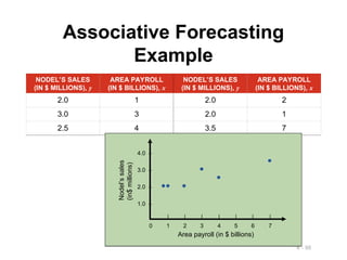
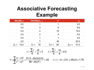
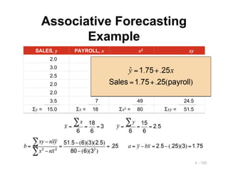
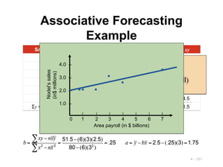
NODEL’S SALES
(IN $ MILLIONS), y
AREA PAYROLL
(IN $ BILLIONS), x
NODEL’S SALES
(IN $ MILLIONS), y
AREA PAYROLL
(IN $ BILLIONS), x
2.0 1 2.0 2
3.0 3 2.0 1
2.5 4 3.5 7
4.0 –
3.0 –
2.0 –
1.0 –
| | | | | | |
0 1 2 3 4 5 6 7
Area payroll (in $ billions)
Nodel’s
sales
(in$
millions)
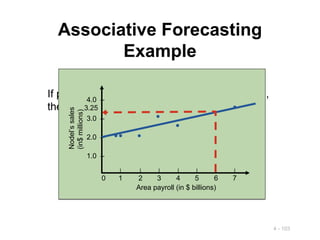
4 - 102
AssociativeForecasting
Example
If payroll next year is estimated to be $6 billion,
then:
Sales (in $ millions) = 1.75 + .25(6)
= 1.75 + 1.5 = 3.25
Sales = $3,250,000
103.
4 - 103
AssociativeForecasting
Example
If payroll next year is estimated to be $6 billion,
then:
Sales (in$ millions) = 1.75 + .25(6)
= 1.75 + 1.5 = 3.25
Sales = $3,250,000
4.0 –
3.0 –
2.0 –
1.0 –
| | | | | | |
0 1 2 3 4 5 6 7
Area payroll (in $ billions)
Nodel’s
sales
(in$
millions)
3.25
104.
4 - 104
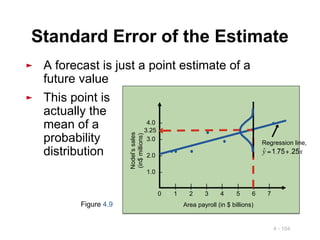
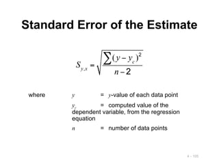
StandardError of the Estimate
► A forecast is just a point estimate of a
future value
► This point is
actually the
mean of a
probability
distribution
Figure 4.9
4.0 –
3.0 –
2.0 –
1.0 –
| | | | | | |
0 1 2 3 4 5 6 7
Area payroll (in $ billions)
Nodel’s
sales
(in$
millions)
3.25
Regression line,
105.
4 - 105
StandardError of the Estimate
where y = y-value of each data point
yc = computed value of the
dependent variable, from the regression
equation
n = number of data points
106.
4 - 106
StandardError of the Estimate
Computationally, this equation is
considerably easier to use
We use the standard error to set up
prediction intervals around the point
estimate
107.
4 - 107
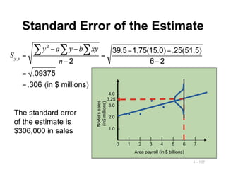
StandardError of the Estimate
The standard error
of the estimate is
$306,000 in sales
4.0 –
3.0 –
2.0 –
1.0 –
| | | | | | |
0 1 2 3 4 5 6 7
Area payroll (in $ billions)
Nodel’s
sales
(in$
millions)
3.25
108.
4 - 108
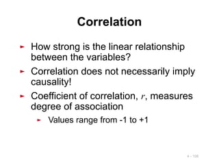
►How strong is the linear relationship
between the variables?
► Correlation does not necessarily imply
causality!
► Coefficient of correlation, r, measures
degree of association
► Values range from -1 to +1
Correlation
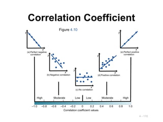
4 - 110
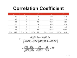
CorrelationCoefficient
y
x
(a) Perfect negative
correlation
y
x
(c) No correlation
y
x
(d) Positive correlation
y
x
(e) Perfect positive
correlation
y
x
(b) Negative correlation
High
Moderate
Low
Correlation coefficient values
High Moderate Low
| | | | | | | | |
–1.0 –0.8 –0.6 –0.4 –0.2 0 0.2 0.4 0.6 0.8 1.0
Figure 4.10
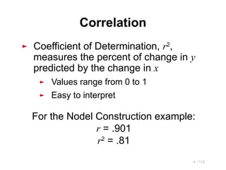
4 - 112
►Coefficient of Determination, r2
,
measures the percent of change in y
predicted by the change in x
► Values range from 0 to 1
► Easy to interpret
Correlation
For the Nodel Construction example:
r = .901
r2
= .81
113.
4 - 113
Multiple-RegressionAnalysis
If more than one independent variable is to be
used in the model, linear regression can be
extended to multiple regression to accommodate
several independent variables
Computationally, this is quite
complex and generally done on the
computer
114.
4 - 114
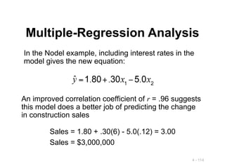
Multiple-RegressionAnalysis
In the Nodel example, including interest rates in the
model gives the new equation:
An improved correlation coefficient of r = .96 suggests
this model does a better job of predicting the change
in construction sales
Sales = 1.80 + .30(6) - 5.0(.12) = 3.00
Sales = $3,000,000
115.
4 - 115
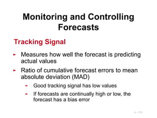
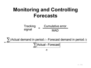
►Measures how well the forecast is predicting
actual values
► Ratio of cumulative forecast errors to mean
absolute deviation (MAD)
► Good tracking signal has low values
► If forecasts are continually high or low, the
forecast has a bias error
Monitoring and Controlling
Forecasts
Tracking Signal
4 - 117
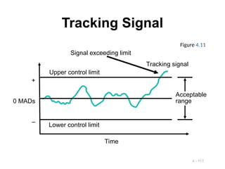
TrackingSignal
Tracking signal
+
0 MADs
–
Upper control limit
Lower control limit
Time
Signal exceeding limit
Acceptable
range
Figure 4.11
118.
4 - 118
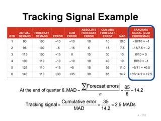
TrackingSignal Example
QTR
ACTUAL
DEMAND
FORECAST
DEMAND ERROR
CUM
ERROR
ABSOLUTE
FORECAST
ERROR
CUM ABS
FORECAST
ERROR MAD
TRACKING
SIGNAL (CUM
ERROR/MAD)
1 90 100 –10 –10 10 10 10.0 –10/10 = –1
2 95 100 –5 –15 5 15 7.5 –15/7.5 = –2
3 115 100 +15 0 15 30 10. 0/10 = 0
4 100 110 –10 –10 10 40 10. 10/10 = –1
5 125 110 +15 +5 15 55 11.0 +5/11 = +0.5
6 140 110 +30 +35 30 85 14.2 +35/14.2 = +2.5
At the end of quarter 6,
119.
4 - 119
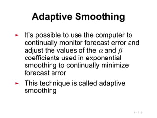
AdaptiveSmoothing
► It’s possible to use the computer to
continually monitor forecast error and
adjust the values of the and
coefficients used in exponential
smoothing to continually minimize
forecast error
► This technique is called adaptive
smoothing
120.
4 - 120
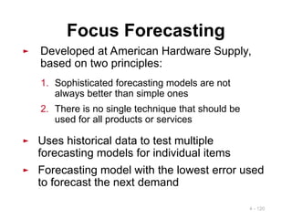
FocusForecasting
► Developed at American Hardware Supply,
based on two principles:
1. Sophisticated forecasting models are not
always better than simple ones
2. There is no single technique that should be
used for all products or services
► Uses historical data to test multiple
forecasting models for individual items
► Forecasting model with the lowest error used
to forecast the next demand
121.
4 - 121
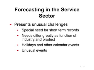
Forecastingin the Service
Sector
► Presents unusual challenges
► Special need for short term records
► Needs differ greatly as function of
industry and product
► Holidays and other calendar events
► Unusual events
122.
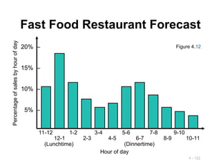
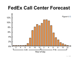
4 - 122
FastFood Restaurant Forecast
20% –
15% –
10% –
5% –
11-12 1-2 3-4 5-6 7-8 9-10
12-1 2-3 4-5 6-7 8-9 10-11
(Lunchtime) (Dinnertime)
Hour of day
Percentage
of
sales
by
hour
of
day
Figure 4.12


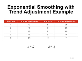
![4 - 40
Weighted Moving Average
MONTH ACTUAL SHED SALES 3-MONTH WEIGHTED MOVING AVERAGE
January 10
February 12
March 13
April 16
May 19
June 23
July 26
August 30
September 28
October 18
November 16
December 14
WEIGHTS APPLIED PERIOD
3 Last month
2 Two months ago
1 Three months ago
6 Sum of the weights
Forecast for this month =
3 x Sales last mo. + 2 x Sales 2 mos. ago + 1 x Sales 3 mos. ago
Sum of the weights
[(3 x 13) + (2 x 12) + (10)]/6 = 12 1
/6
10
12
13](https://image.slidesharecdn.com/forecasting-250817074705-3290aa37/85/hr_om11_ch03_project-FORECASTING-ppts-for-forecasting-40-320.jpg)
![4 - 41
Weighted Moving Average
MONTH ACTUAL SHED SALES 3-MONTH WEIGHTED MOVING AVERAGE
January 10
February 12
March 13
April 16
May 19
June 23
July 26
August 30
September 28
October 18
November 16
December 14
[(3 x 13) + (2 x 12) + (10)]/6 = 12 1
/6
10
12
13
[(3 x 16) + (2 x 13) + (12)]/6 = 14 1
/3
[(3 x 19) + (2 x 16) + (13)]/6 = 17
[(3 x 23) + (2 x 19) + (16)]/6 = 20 1
/2
[(3 x 26) + (2 x 23) + (19)]/6 = 23 5
/6
[(3 x 30) + (2 x 26) + (23)]/6 = 27 1
/2
[(3 x 28) + (2 x 30) + (26)]/6 = 28 1
/3
[(3 x 18) + (2 x 28) + (30)]/6 = 23 1
/3
[(3 x 16) + (2 x 18) + (28)]/6 = 18 2
/3](https://image.slidesharecdn.com/forecasting-250817074705-3290aa37/85/hr_om11_ch03_project-FORECASTING-ppts-for-forecasting-41-320.jpg)


![Product1 [3] forecasting v2](https://cdn.slidesharecdn.com/ss_thumbnails/product13-forecastingv2-190226041012-thumbnail.jpg?width=640&height=640&fit=bounds)