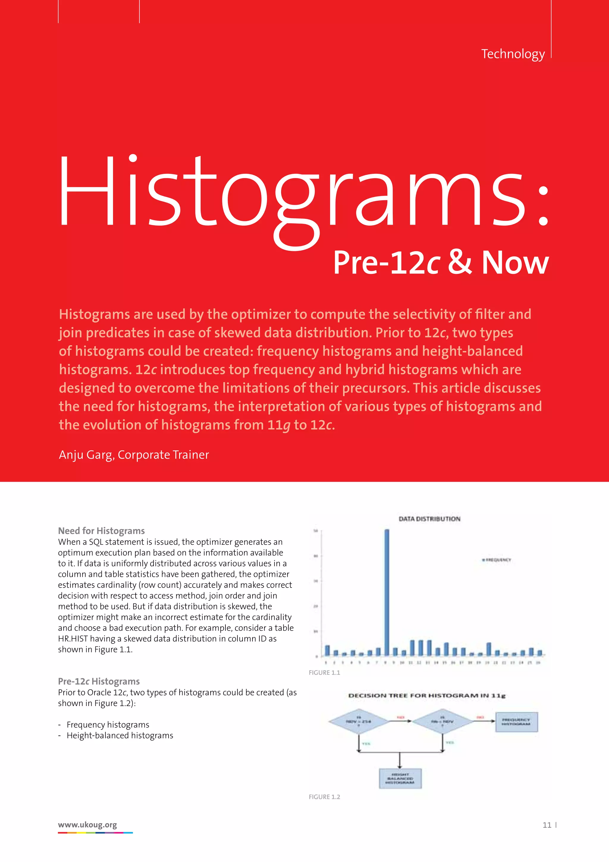
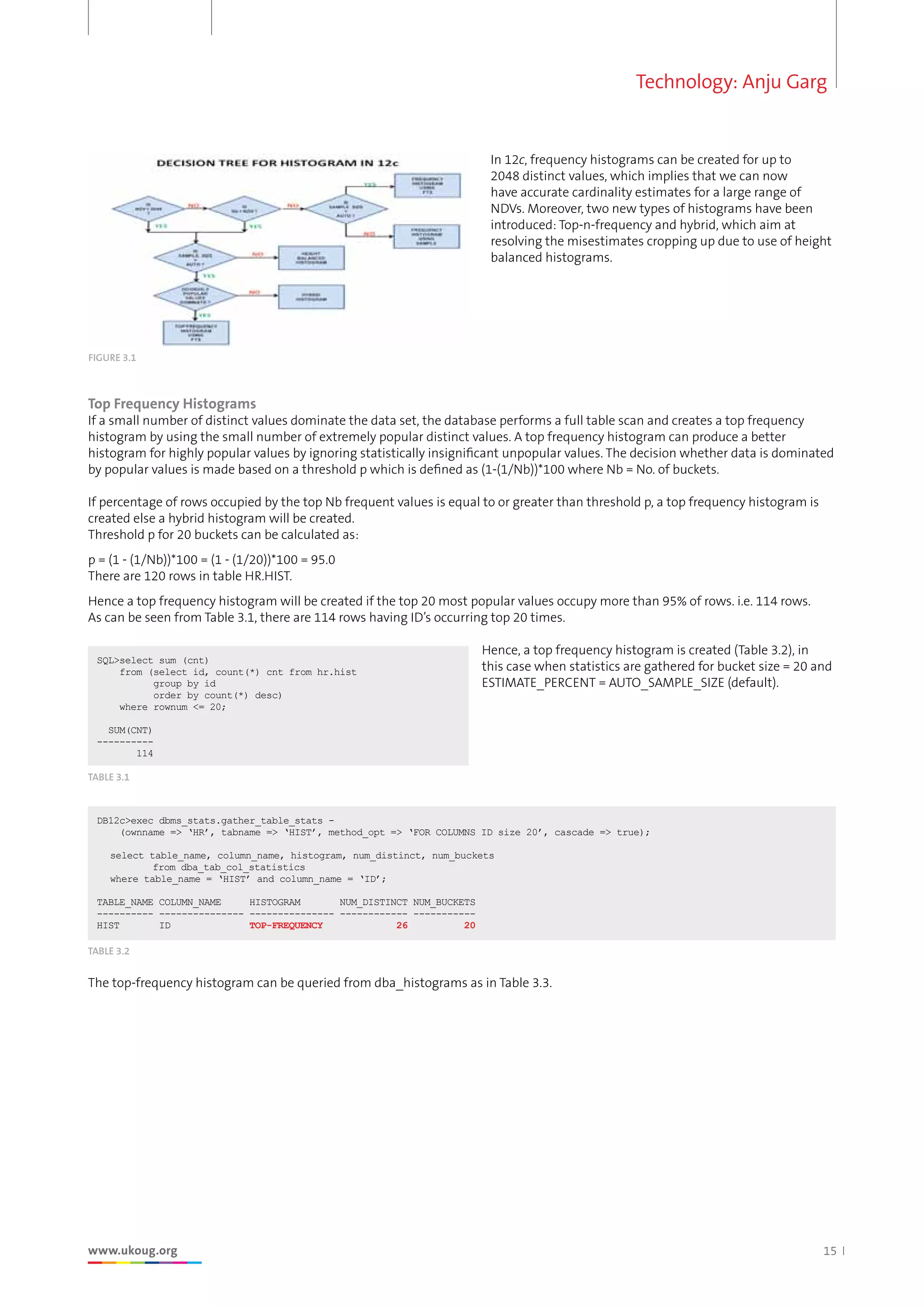
SlideShare a Scribd company logo
1 of 8
Header here
www.ukoug.org 11
Histograms:
Histograms are used by the optimizer to compute the selectivity of filter and
join predicates in case of skewed data distribution. Prior to 12c, two types
of histograms could be created: frequency histograms and height-balanced
histograms. 12c introduces top frequency and hybrid histograms which are
designed to overcome the limitations of their precursors. This article discusses
the need for histograms, the interpretation of various types of histograms and
the evolution of histograms from 11g to 12c.
Anju Garg, Corporate Trainer
Pre-12c & Now
Need for Histograms
When a SQL statement is issued, the optimizer generates an
optimum execution plan based on the information available
to it. If data is uniformly distributed across various values in a
column and table statistics have been gathered, the optimizer
estimates cardinality (row count) accurately and makes correct
decision with respect to access method, join order and join
method to be used. But if data distribution is skewed, the
optimizer might make an incorrect estimate for the cardinality
and choose a bad execution path. For example, consider a table
HR.HIST having a skewed data distribution in column ID as
shown in Figure 1.1.
Pre-12c Histograms
Prior to Oracle 12c, two types of histograms could be created (as
shown in Figure 1.2):
-	 Frequency histograms
-	 Height-balanced histograms
Technology
FIGURE 1.1
FIGURE 1.2
12 www.ukoug.org
SUMMER 15
Technology: Anju Garg
OracleScene
D I G I T A L
Frequency Histograms
A frequency histogram is a frequency distribution which records each different value and its exact cardinality. A frequency
histogram is created when
-	Requested no. of buckets (Nb) = No. of distinct values (NDV) and
-	 NDV = 254 (2,048 in 12c).
A frequency histogram with 26 buckets for ID column can be created as under:
TABLE 2.1
SQLexec dbms_stats.gather_table_stats -
(ownname = ‘HR’,tabname = ‘HIST’,method_opt = ‘FOR COLUMNS ID’, cascade = true);
SQL select table_name, column_name, histogram, num_distinct, num_buckets
from dba_tab_col_statistics
where table_name = ‘HIST’ and column_name = ‘ID’;
TABLE_NAME COLUMN_NAME HISTOGRAM NUM_DISTINCT NUM_BUCKETS
---------- --------------- --------------- ------------ -----------
HIST ID FREQUENCY 26 26
The histogram can be viewed from DBA_HISTOGRAMS (as shown in Table 2.2)
SQL select ENDPOINT_VALUE, ENDPOINT_NUMBER
from dba_histograms
where table_name = ‘HIST’
and column_name = ‘ID’;
ENDPOINT_VALUE ENDPOINT_NUMBER
-------------- ---------------
1 4
2 6
3 7
4 9
5 10
6 12
7 15
8 65
9 68
10 70
11 76
12 82
13 88
14 91
15 96
16 99
17 102
18 103
19 104
20 109
21 111
22 112
23 113
24 115
25 118
26 120
TABLE 2.2
FIGURE 2.2
Interpreting Frequency Histogram
It can be seen from Table 2.2 that a frequency histogram with 26 buckets, one for each distinct value, has been created.
•	 ENDPOINT_VALUE - The value in a bucket.
•	 ENDPOINT_NUMBER - Cumulative frequency
Thus, you can find out the exact counts for each of the distinct values in the data. For example, the optimizer makes an accurate
estimate of 50 rows for ID = 8 and uses FTS access path as desired (Table 2.3) even though column ID is indexed.
TABLE 2.3
SQLexplain plan for select * from hr.hist where id = 8;
select * from table(dbms_xplan.display);
PLAN_TABLE_OUTPUT
---------------------------------------------------------------------------------Plan hash value: 538080257
--------------------------------------------------------------------------
| Id | Operation | Name | Rows | Bytes | Cost (%CPU)| Time |
--------------------------------------------------------------------------
| 0 | SELECT STATEMENT | | 50 | 50200 | 7 (0)| 00:00:01 |
|* 1 | TABLE ACCESS FULL| HIST | 50 | 50200 | 7 (0)| 00:00:01 |
--------------------------------------------------------------------------
Technology: Anju Garg
www.ukoug.org 13
Thus, prior to 12c, frequency histograms could be used to accurately estimate the frequencies if NDV = 254.
Height-balanced Histograms
A height-balanced histogram is created if NDV  254 or Nb  NDV. This histogram distributes the count of all rows evenly across
all histogram buckets, so all buckets will have almost exactly the same number of rows. A height-balanced histogram is much less
precise and can’t really capture information about more than 127 popular values.
To create height balanced histogram, specify no. of buckets = 20 ( NDV (=26) )
DB11gexec dbms_stats.gather_table_stats -
(ownname = ‘HR’, tabname = ‘HIST’,method_opt = ‘FOR COLUMNS ID size 20’, cascade = true);
It can be seen that the height-balanced histogram has been created as No. of buckets (20)  NDV (26) (Table 2.4).
DB11gselect table_name, column_name, histogram, num_distinct, num_buckets
from dba_tab_col_statistics
where table_name = ‘HIST’ and column_name = ‘ID’;
TABLE_NAME COLUMN_NAME HISTOGRAM NUM_DISTINCT NUM_BUCKETS
---------- --------------- --------------- ------------ -----------
HIST ID HEIGHT BALANCED 26 20
TABLE 2.4
The height-balanced histogram that has been created can be viewed in Table 2.5.
DB11gselect ENDPOINT_VALUE, ENDPOINT_NUMBER
from dba_histograms
where table_name = ‘HIST’
and column_name = ‘ID’;
ENDPOINT_VALUE ENDPOINT_NUMBER
-------------- --------------
1 0
2 1
6 2
8 10
9 11
11 12
12 13
13 14
14 15
15 16
17 17
20 18
24 19
26 20
14 rows selected.
TABLE 2.5 FIGURE 2.3
Interpreting Height-balanced Histogram
•	 Bucket size = Total no. of rows / Nb = 120 / 20 = 6
•	 ENDPOINT_NUMBER - A number uniquely identifying a bucket
•	 For bucket with ENDPOINT_NUMBER 0, ENDPOINT_VALUE = the lowest value (1 here)
•	 For buckets with ENDPOINT_NUMBER  0, ENDPOINT_VALUE = largest value stored in that bucket
Note that when storing the histogram selection, Oracle doesn’t store repetitions of end point values. If there are multiple buckets
with same end points, only one bucket is stored with its highest end point number. For example, there are 8 buckets (3 - 10)
containing the value 8. The histogram stores only one entry with the highest ENDPOINT_NUMBER, i.e. 10.
The optimizer decides the popularity of a value by the number of buckets having that value as its end point. Since value 8 is the
endpoint of multiple buckets, it is considered as a popular value. The cardinality of a popular value is derived as the product of
bucket size and the number of buckets having the value as their end point. For example, cardinality for value 8 = no. of buckets
having 8 as end point * bucket size i.e. 8 * 6 = 48 (actual = 50).
14 www.ukoug.org
SUMMER 15
Technology: Anju Garg
OracleScene
D I G I T A L
TABLE 2.6
DB11g explain plan for select * from hr.hist where id =8;
select * from table(dbms_xplan.display);
PLAN_TABLE_OUTPUT
--------------------------------------------------------------------------------
Plan hash value: 538080257
--------------------------------------------------------------------------
| Id | Operation | Name | Rows | Bytes | Cost (%CPU)| Time |
--------------------------------------------------------------------------
| 0 | SELECT STATEMENT | | 48 | 48192 | 7 (0)| 00:00:01 |
|* 1 | TABLE ACCESS FULL| HIST | 48 | 48192 | 7 (0)| 00:00:01 |
--------------------------------------------------------------------------
Predicate Information (identified by operation id):
---------------------------------------------------
2 - access(“ID”=8)
If we search for an unpopular value i.e. the value which is not an end point or is the end point of only one bucket, the optimizer
calculates the cardinality as (number of rows in table)*density where density is calculated by the optimizer using an internal
algorithm based on factors such as the number of buckets and the NDV. For example, consider two unpopular values:
ID = 15 occurs 5 times and is an end point of one bucket
ID = 3 occurs once and is not an end point
It can be seen that the number of rows estimated for both the unpopular values is same i.e. 3 (Table 2.7 and Table 2.8).
TABLE 2.7
DB11gexplain plan for select * from hr.hist where id = 15;
select * from table(dbms_xplan.display);
PLAN_TABLE_OUTPUT
---------------------------------------------------------------------------------
Plan hash value: 4058847011
---------------------------------------------------------------------------------
| Id | Operation | Name | Rows | Bytes | Cost (%CPU)|Time
---------------------------------------------------------------------------------
| 0 | SELECT STATEMENT | | 3 | 3012 | 2 (0)| 00:00:01
| 1 | TABLE ACCESS BY INDEX ROWID| HIST | 3 | 3012 | 2 (0)| 00:00:01
|* 2 | INDEX RANGE SCAN | HIST_IDX | 3 | | 1 (0)| 00:00:01
---------------------------------------------------------------------------------
Predicate Information (identified by operation id):
---------------------------------------------------
2 - access(“ID”=15)
TABLE 2.8
DB11gexplain plan for select * from hr.hist where id = 3;
select * from table(dbms_xplan.display);
PLAN_TABLE_OUTPUT
---------------------------------------------------------------------------------
Plan hash value: 4058847011
---------------------------------------------------------------------------------
| Id | Operation | Name | Rows | Bytes |Cost (%CPU)| Time
---------------------------------------------------------------------------------
| 0 | SELECT STATEMENT | | 3 | 3012 | 2 (0)| 00:00:01
| 1 | TABLE ACCESS BY INDEX ROWID| HIST | 3 | 3012 | 2 (0)| 00:00:01
|* 2 | INDEX RANGE SCAN | HIST_IDX | 3 | | 1 (0)| 00:00:01
---------------------------------------------------------------------------------
Predicate Information (identified by operation id):
---------------------------------------------------
2 - access”ID”=3)
Hence, it can be inferred that height-balanced histograms simply decide the cardinality of value based on the popularity of a value
which depends on the number of buckets having the value as end point.
Issues with Histograms in 11g
- Frequency histograms are accurate, but can be created only for NDV = 254
- Height-balanced histograms may cause the optimizer to choose a suboptimal plan in cases where a value is an end point of only
one bucket, but almost fills up another bucket. In such a scenario the value might be considered unpopular.
Technology: Anju Garg
www.ukoug.org 15
In 12c, frequency histograms can be created for up to
2048 distinct values, which implies that we can now
have accurate cardinality estimates for a large range of
NDVs. Moreover, two new types of histograms have been
introduced: Top-n-frequency and hybrid, which aim at
resolving the misestimates cropping up due to use of height
balanced histograms.
Top Frequency Histograms
If a small number of distinct values dominate the data set, the database performs a full table scan and creates a top frequency
histogram by using the small number of extremely popular distinct values. A top frequency histogram can produce a better
histogram for highly popular values by ignoring statistically insignificant unpopular values. The decision whether data is dominated
by popular values is made based on a threshold p which is defined as (1-(1/Nb))*100 where Nb = No. of buckets.
If percentage of rows occupied by the top Nb frequent values is equal to or greater than threshold p, a top frequency histogram is
created else a hybrid histogram will be created.
Threshold p for 20 buckets can be calculated as:
p = (1 - (1/Nb))*100 = (1 - (1/20))*100 = 95.0
There are 120 rows in table HR.HIST.
Hence a top frequency histogram will be created if the top 20 most popular values occupy more than 95% of rows. i.e. 114 rows.
As can be seen from Table 3.1, there are 114 rows having ID’s occurring top 20 times.
Hence, a top frequency histogram is created (Table 3.2), in
this case when statistics are gathered for bucket size = 20 and
ESTIMATE_PERCENT = AUTO_SAMPLE_SIZE (default).
TABLE 3.2
DB12cexec dbms_stats.gather_table_stats -
(ownname = ‘HR’, tabname = ‘HIST’, method_opt = ‘FOR COLUMNS ID size 20’, cascade = true);
	 select table_name, column_name, histogram, num_distinct, num_buckets
	 from dba_tab_col_statistics
	 where table_name = ‘HIST’ and column_name = ‘ID’;
TABLE_NAME COLUMN_NAME HISTOGRAM NUM_DISTINCT NUM_BUCKETS
---------- --------------- --------------- ------------ -----------
HIST ID TOP-FREQUENCY 26 20
The top-frequency histogram can be queried from dba_histograms as in Table 3.3.
FIGURE 3.1
TABLE 3.1
SQLselect sum (cnt)
from (select id, count(*) cnt from hr.hist
group by id
order by count(*) desc)
where rownum = 20;
SUM(CNT)
----------
114
16 www.ukoug.org
SUMMER 15
Technology: Anju Garg
OracleScene
D I G I T A L
DB12cselect ENDPOINT_VALUE, ENDPOINT_NUMBER
	 from dba_histograms
	 where table_name = ‘HIST’
	 and column_name = ‘ID’;
ENDPOINT_VALUE ENDPOINT_NUMBER
-------------- ---------------
1 4
2 6
4 8
6 10
7 13
8 63
9 66
10 68
11 74
12 80
13 86
14 89
15 94
16 97
17 100
20 105
21 107
24 109
25 112
26 114
20 rows selected
TABLE 3.3 FIGURE 3.2
Interpreting Top Frequency Histogram
•	 ENDPOINT_VALUE represents key value (ID)
•	 ENDPOINT_NUMBER represents cumulative frequency
•	 Since NDV (26)  Nb (20), only 20 values are captured which occur most frequently
•	 Frequencies of least occurring 6 values (bottom 5%) have not been stored
It can be seen that a top frequency histogram makes an accurate cardinality estimate for both id = 15 (Table 3.4) and 3 (Table 3.5)
which were considered non-popular values in the height-balanced histogram.
TABLE 3.4
DB12cexplain plan for select * from hr.hist where id = 15;
select * from table(dbms_xplan.display);
PLAN_TABLE_OUTPUT
---------------------------------------------------------------------------------
Plan hash value: 3950962134
---------------------------------------------------------------------------------
| Id | Operation | Name | Rows | Bytes | Cost (%CPU)| Time |
---------------------------------------------------------------------------------
| 0 | SELECT STATEMENT | | 5 |5020 | 2 (0)| 00:00:01
| 1 | TABLE ACCESS BY INDEX ROWID BATCHED| HIST | 5 |5020 | 2 (0)| 00:00:01
|* 2 | INDEX RANGE SCAN |HIST_IDX| 5 | | 1 (0)| 00:00:01
---------------------------------------------------------------------------------
Predicate Information (identified by operation id):
---------------------------------------------------
2 - access(“ID”=15)
TABLE 3.5
DB12cexplain plan for select * from hr.hist where id = 3;
select * from table(dbms_xplan.display);
PLAN_TABLE_OUTPUT
---------------------------------------------------------------------------------
Plan hash value: 3950962134
---------------------------------------------------------------------------------| Id | Operation |
Name |Rows| Bytes|Cost(%CPU)|Time
---------------------------------------------------------------------------------
| 0 | SELECT STATEMENT | | 1 |1004 | 2 (0)| 00:00:01
| 1 | TABLE ACCESS BY INDEX ROWID BATCHED|HIST | 1 |1004 | 2 (0)| 00:00:01
|* 2 | INDEX RANGE SCAN |HIST_IDX| 1 | | 1 (0)| 00:00:01
---------------------------------------------------------------------------------
Predicate Information (identified by operation id):
---------------------------------------------------
2 - access(“ID”=3)
Thus the problem with height balanced histograms, of not being able to estimate the frequency of unpopular values accurately,
has been resolved by top frequency histograms in cases when a small number of distinct values dominate the majority of distinct
values. This histogram is gathered using a full table scan of a table. The occurrences of popular values are accurately captured at the
expense of not capturing the data for least occurring values.
Technology: Anju Garg
www.ukoug.org 17
Hybrid Histograms
A hybrid histogram is so called as it combines the characteristics of both height-based histograms and frequency histograms. As we
saw earlier, the height-balanced histogram may produce inaccurate estimates for:
•	 a value that is not an end point
•	 a value that is an end point of only one bucket
•	 a value that is an end point of multiple buckets and almost fills up the last bucket
A hybrid histogram attempts to overcome above shortcomings as it has following features:
•	For each end point in the histogram, it stores the ENDPOINT_REPEAT_COUNT value, which is the number of times the end point
value is repeated. Thus, it has an accurate frequency of end point values.
•	As compared to a height-balanced histogram where a value having frequency greater than bucket size could be spread across
multiple buckets, a hybrid histogram stores all the occurrences of every value in the same bucket, i.e. a value cannot span
multiple buckets. As a result, it can capture more end points.
•	Similar to a height-balanced histogram, a bucket in a hybrid histogram can contain more than one value.
An after effect of this implementation is variable bucket size. Since each value possibly having a different frequency will be
contained entirely in one bucket only and one bucket can even have more than one value, buckets of different size may result.
A histogram with 20 buckets will be created as a hybrid histogram if rows having top 20 most popular IDs are less than threshold p
for 20 buckets.
p = (1 - (1/nb))*100 = (1 - (1/20))*100 = 95.0
On deleting 20 rows with ID = 8 from table HR.HIST, it qualifies for hybrid histogram creation as no. of rows having id’s occurring top
20 times = 94 (Table 3.7) which is less than 95% of rows. i.e. 95 rows.
TABLE 3.6
DB12cdelete from hr.hist where id = 8 and rownum =20;
commit;
select count(*) from hr.hist;
COUNT(*)
----------
100
TABLE 3.7
DB12cselect sum (cnt)
from (select id, count(*) cnt from hr.hist
group by id
order by count(*) desc)
where rownum = 20;
SUM(CNT)
----------
94
It can be seen from that, a hybrid histogram with 20 buckets has been created (Table 3.8 and Table 3.9).
TABLE 3.8
DB12cexec dbms_stats.gather_table_stats -
(ownname = ‘HR’,tabname = ‘HIST’, method_opt = ‘FOR COLUMNS ID size 20’, cascade = true);
DB12c select table_name, column_name, histogram, num_distinct, num_buckets
	 from dba_tab_col_statistics
	 where table_name = ‘HIST’ and column_name = ‘ID’;
TABLE_NAME COLUMN_NAME HISTOGRAM NUM_DISTINCT NUM_BUCKETS
---------- --------------- --------------- ------------ -----------
HIST ID HYBRID 26 20
DB12cselect ENDPOINT_VALUE, ENDPOINT_NUMBER,
ENDPOINT_REPEAT_COUNT RPT_CNT
	 from dba_histograms
	 where table_name = ‘HIST’
	 and column_name = ‘ID’;
ENDPOINT_VALUE ENDPOINT_NUMBER RPT_CNT
-------------- --------------- ----------
1 4 4
3 7 1
5 10 1
7 15 3
8 45 30
10 50 2
11 56 6
12 62 6
13 68 6
14 71 3
15 76 5
16 79 3
17 82 3
19 84 1
20 89 5
21 91 2
22 92 1
23 93 1
24 95 2
26 100 2
20 rows selected.
TABLE 3.9
18 www.ukoug.org
SUMMER 15
Technology: Anju Garg
OracleScene
D I G I T A L
Interpreting Hybrid Histogram
•	 ENDPOINT_VALUE: The largest value in a bucket
•	 ENDPOINT_NUMBER: Cumulative frequency.
	 The difference of 2 consecutive ENDPOINT_NUMBER’s gives
	 the bucket size.
•	 ENDPOINT_REPEAT_COUNT: Frequency of endpoint
Based on the above information, data has been arranged in buckets as shown in fig 3.3. It can be seen that Hybrid histogram
captures more endpoints (20 = Nb) as compared to Height Balanced histogram (14) and can estimate their cardinality accurately.
Thus, it is evident that Hybrid histograms have features of both frequency and height balanced histograms. Features similar to
frequency histograms:
•	 All occurrences of a value are placed in one bucket
•	 ENDPOINT_NUMBER stores cumulative frequency
Features similar to height-balanced histograms:
•	 One bucket can contain multiple values.
FIGURE 3.3
Summary
•	 In 12c, a frequency histogram can be created for NDV = 2048.
•	 Top frequency and hybrid histograms are designed to overcome flaws of height-balanced histograms.
•	 Top frequency and hybrid histograms are created only if ESTIMATE_PERCENT = AUTO_SAMPLE_SIZE.
•	Top frequency histograms accurately estimate the frequencies for only top occurring values if a small number of values
dominate the data set.
•	 Hybrid histograms have features of both frequency and height-balanced histograms
•	Hybrid histograms capture more end points as compared to height-balanced histograms and estimate their frequency
accurately.
References
•	 http://docs.oracle.com/database/121/TGSQL/tgsql_histo.htm#TGSQL366
•	 http://jimczuprynski.files.wordpress.com/2014/04/czuprynski-select-q2-2014.pdf
•	 http://jonathanlewis.wordpress.com/2013/09/01/histograms/
ABOUT
THE
AUTHOR
Anju Garg
Corporate Trainer
Anju Garg is an Oracle Ace Associate with over 12 years of experience in the IT industry in
various roles. Since 2010, she has been involved in teaching and has trained more than
100 DBAs from across the world in various core DBA technologies like RAC, Data guard,
Performance Tuning, SQL statement tuning, Database Administration etc. Anju is
passionate about learning and has a keen interest in RAC and Performance Tuning,
sharing her knowledge via her technical blog.
Blog: 	 http://oracleinaction.com

More Related Content

What's hot

Optimizer Trace Walkthrough
Optimizer Trace WalkthroughOptimizer Trace Walkthrough
Optimizer Trace WalkthroughSergey Petrunya
 
Basic Query Tuning Primer - Pg West 2009
Basic Query Tuning Primer - Pg West 2009Basic Query Tuning Primer - Pg West 2009
Basic Query Tuning Primer - Pg West 2009mattsmiley
 
A few things about the Oracle optimizer - 2013
A few things about the Oracle optimizer - 2013A few things about the Oracle optimizer - 2013
A few things about the Oracle optimizer - 2013Connor McDonald
 
Oracle Parallel Distribution and 12c Adaptive Plans
Oracle Parallel Distribution and 12c Adaptive PlansOracle Parallel Distribution and 12c Adaptive Plans
Oracle Parallel Distribution and 12c Adaptive PlansFranck Pachot
 
Explaining the Postgres Query Optimizer
Explaining the Postgres Query OptimizerExplaining the Postgres Query Optimizer
Explaining the Postgres Query OptimizerEDB
 
Using histograms to get better performance
Using histograms to get better performanceUsing histograms to get better performance
Using histograms to get better performanceSergey Petrunya
 
Lessons for the optimizer from running the TPC-DS benchmark
Lessons for the optimizer from running the TPC-DS benchmarkLessons for the optimizer from running the TPC-DS benchmark
Lessons for the optimizer from running the TPC-DS benchmarkSergey Petrunya
 
Full Table Scan: friend or foe
Full Table Scan: friend or foeFull Table Scan: friend or foe
Full Table Scan: friend or foeMauro Pagano
 
Star Transformation, 12c Adaptive Bitmap Pruning and In-Memory option
Star Transformation, 12c Adaptive Bitmap Pruning and In-Memory optionStar Transformation, 12c Adaptive Bitmap Pruning and In-Memory option
Star Transformation, 12c Adaptive Bitmap Pruning and In-Memory optionFranck Pachot
 
SQL Macros - Game Changing Feature for SQL Developers?
SQL Macros - Game Changing Feature for SQL Developers?SQL Macros - Game Changing Feature for SQL Developers?
SQL Macros - Game Changing Feature for SQL Developers?Andrej Pashchenko
 
Oracle statistics by example
Oracle statistics by exampleOracle statistics by example
Oracle statistics by exampleMauro Pagano
 
Optimizer features in recent releases of other databases
Optimizer features in recent releases of other databasesOptimizer features in recent releases of other databases
Optimizer features in recent releases of other databasesSergey Petrunya
 
ANALYZE for Statements - MariaDB's hidden gem
ANALYZE for Statements - MariaDB's hidden gemANALYZE for Statements - MariaDB's hidden gem
ANALYZE for Statements - MariaDB's hidden gemSergey Petrunya
 
Common Table Expressions in MariaDB 10.2 (Percona Live Amsterdam 2016)
Common Table Expressions in MariaDB 10.2 (Percona Live Amsterdam 2016)Common Table Expressions in MariaDB 10.2 (Percona Live Amsterdam 2016)
Common Table Expressions in MariaDB 10.2 (Percona Live Amsterdam 2016)Sergey Petrunya
 
How the Postgres Query Optimizer Works
How the Postgres Query Optimizer WorksHow the Postgres Query Optimizer Works
How the Postgres Query Optimizer WorksEDB
 
CBO Basics: Cardinality
CBO Basics: CardinalityCBO Basics: Cardinality
CBO Basics: CardinalitySidney Chen
 
Checking clustering factor to detect row migration
Checking clustering factor to detect row migrationChecking clustering factor to detect row migration
Checking clustering factor to detect row migrationHeribertus Bramundito
 

What's hot (19)

Optimizer Trace Walkthrough
Optimizer Trace WalkthroughOptimizer Trace Walkthrough
Optimizer Trace Walkthrough
 
Basic Query Tuning Primer - Pg West 2009
Basic Query Tuning Primer - Pg West 2009Basic Query Tuning Primer - Pg West 2009
Basic Query Tuning Primer - Pg West 2009
 
Oracle 12c SPM
Oracle 12c SPMOracle 12c SPM
Oracle 12c SPM
 
A few things about the Oracle optimizer - 2013
A few things about the Oracle optimizer - 2013A few things about the Oracle optimizer - 2013
A few things about the Oracle optimizer - 2013
 
Oracle Parallel Distribution and 12c Adaptive Plans
Oracle Parallel Distribution and 12c Adaptive PlansOracle Parallel Distribution and 12c Adaptive Plans
Oracle Parallel Distribution and 12c Adaptive Plans
 
Explaining the Postgres Query Optimizer
Explaining the Postgres Query OptimizerExplaining the Postgres Query Optimizer
Explaining the Postgres Query Optimizer
 
Using histograms to get better performance
Using histograms to get better performanceUsing histograms to get better performance
Using histograms to get better performance
 
Lessons for the optimizer from running the TPC-DS benchmark
Lessons for the optimizer from running the TPC-DS benchmarkLessons for the optimizer from running the TPC-DS benchmark
Lessons for the optimizer from running the TPC-DS benchmark
 
Full Table Scan: friend or foe
Full Table Scan: friend or foeFull Table Scan: friend or foe
Full Table Scan: friend or foe
 
The PostgreSQL Query Planner
The PostgreSQL Query PlannerThe PostgreSQL Query Planner
The PostgreSQL Query Planner
 
Star Transformation, 12c Adaptive Bitmap Pruning and In-Memory option
Star Transformation, 12c Adaptive Bitmap Pruning and In-Memory optionStar Transformation, 12c Adaptive Bitmap Pruning and In-Memory option
Star Transformation, 12c Adaptive Bitmap Pruning and In-Memory option
 
SQL Macros - Game Changing Feature for SQL Developers?
SQL Macros - Game Changing Feature for SQL Developers?SQL Macros - Game Changing Feature for SQL Developers?
SQL Macros - Game Changing Feature for SQL Developers?
 
Oracle statistics by example
Oracle statistics by exampleOracle statistics by example
Oracle statistics by example
 
Optimizer features in recent releases of other databases
Optimizer features in recent releases of other databasesOptimizer features in recent releases of other databases
Optimizer features in recent releases of other databases
 
ANALYZE for Statements - MariaDB's hidden gem
ANALYZE for Statements - MariaDB's hidden gemANALYZE for Statements - MariaDB's hidden gem
ANALYZE for Statements - MariaDB's hidden gem
 
Common Table Expressions in MariaDB 10.2 (Percona Live Amsterdam 2016)
Common Table Expressions in MariaDB 10.2 (Percona Live Amsterdam 2016)Common Table Expressions in MariaDB 10.2 (Percona Live Amsterdam 2016)
Common Table Expressions in MariaDB 10.2 (Percona Live Amsterdam 2016)
 
How the Postgres Query Optimizer Works
How the Postgres Query Optimizer WorksHow the Postgres Query Optimizer Works
How the Postgres Query Optimizer Works
 
CBO Basics: Cardinality
CBO Basics: CardinalityCBO Basics: Cardinality
CBO Basics: Cardinality
 
Checking clustering factor to detect row migration
Checking clustering factor to detect row migrationChecking clustering factor to detect row migration
Checking clustering factor to detect row migration
 

Viewers also liked

Oracle ACFS High Availability NFS Services (HANFS) Part-I
Oracle ACFS High Availability NFS Services (HANFS) Part-IOracle ACFS High Availability NFS Services (HANFS) Part-I
Oracle ACFS High Availability NFS Services (HANFS) Part-IAnju Garg
 
Oracle ACFS High Availability NFS Services (HANFS)
Oracle ACFS High Availability NFS Services (HANFS)Oracle ACFS High Availability NFS Services (HANFS)
Oracle ACFS High Availability NFS Services (HANFS)Anju Garg
 
Adop and maintenance task presentation 151015
Adop and maintenance task presentation 151015Adop and maintenance task presentation 151015
Adop and maintenance task presentation 151015andreas kuncoro
 
AOUG_11Nov2016_Challenges_with_EBS12_2
AOUG_11Nov2016_Challenges_with_EBS12_2AOUG_11Nov2016_Challenges_with_EBS12_2
AOUG_11Nov2016_Challenges_with_EBS12_2Sean Braymen
 
E business suite r12.2 changes for database administrators
E business suite r12.2 changes for database administratorsE business suite r12.2 changes for database administrators
E business suite r12.2 changes for database administratorsSrinivasa Pavan Marti
 
Oracle RAC, Data Guard, and Pluggable Databases: When MAA Meets Multitenant (...
Oracle RAC, Data Guard, and Pluggable Databases: When MAA Meets Multitenant (...Oracle RAC, Data Guard, and Pluggable Databases: When MAA Meets Multitenant (...
Oracle RAC, Data Guard, and Pluggable Databases: When MAA Meets Multitenant (...Ludovico Caldara
 
Oracle Weblogic for EBS and obiee (R12.2)
Oracle Weblogic for EBS and obiee (R12.2)Oracle Weblogic for EBS and obiee (R12.2)
Oracle Weblogic for EBS and obiee (R12.2)Berry Clemens
 
Policy based cluster management in oracle 12c
Policy based cluster management in oracle 12c Policy based cluster management in oracle 12c
Policy based cluster management in oracle 12c Anju Garg
 
Indexes and Indexing in Oracle 12c
Indexes and Indexing in Oracle 12cIndexes and Indexing in Oracle 12c
Indexes and Indexing in Oracle 12cOren Nakdimon
 
Oracle E-Business Suite R12.2.5 on Database 12c: Install, Patch and Administer
Oracle E-Business Suite R12.2.5 on Database 12c: Install, Patch and AdministerOracle E-Business Suite R12.2.5 on Database 12c: Install, Patch and Administer
Oracle E-Business Suite R12.2.5 on Database 12c: Install, Patch and AdministerAndrejs Karpovs
 
EBS-technical_upgrade_best_practices 12.1 or 12.2
EBS-technical_upgrade_best_practices 12.1 or 12.2EBS-technical_upgrade_best_practices 12.1 or 12.2
EBS-technical_upgrade_best_practices 12.1 or 12.2Berry Clemens
 
Oracle EBS Upgrade to 12.2.5.1
Oracle EBS Upgrade to 12.2.5.1Oracle EBS Upgrade to 12.2.5.1
Oracle EBS Upgrade to 12.2.5.1Amit Sharma
 
Oracle e-business suite R12 step by step Installation
Oracle e-business suite R12 step by step InstallationOracle e-business suite R12 step by step Installation
Oracle e-business suite R12 step by step InstallationOraERP
 
Oracle EBS R12.2 - Deployment and System Administration
Oracle EBS R12.2 - Deployment and System AdministrationOracle EBS R12.2 - Deployment and System Administration
Oracle EBS R12.2 - Deployment and System AdministrationMozammel Hoque
 
Oracle RAC 12c Release 2 - Overview
Oracle RAC 12c Release 2 - OverviewOracle RAC 12c Release 2 - Overview
Oracle RAC 12c Release 2 - OverviewMarkus Michalewicz
 

Viewers also liked (16)

Oracle ACFS High Availability NFS Services (HANFS) Part-I
Oracle ACFS High Availability NFS Services (HANFS) Part-IOracle ACFS High Availability NFS Services (HANFS) Part-I
Oracle ACFS High Availability NFS Services (HANFS) Part-I
 
Oracle ACFS High Availability NFS Services (HANFS)
Oracle ACFS High Availability NFS Services (HANFS)Oracle ACFS High Availability NFS Services (HANFS)
Oracle ACFS High Availability NFS Services (HANFS)
 
Adop and maintenance task presentation 151015
Adop and maintenance task presentation 151015Adop and maintenance task presentation 151015
Adop and maintenance task presentation 151015
 
AOUG_11Nov2016_Challenges_with_EBS12_2
AOUG_11Nov2016_Challenges_with_EBS12_2AOUG_11Nov2016_Challenges_with_EBS12_2
AOUG_11Nov2016_Challenges_with_EBS12_2
 
E business suite r12.2 changes for database administrators
E business suite r12.2 changes for database administratorsE business suite r12.2 changes for database administrators
E business suite r12.2 changes for database administrators
 
Oracle RAC, Data Guard, and Pluggable Databases: When MAA Meets Multitenant (...
Oracle RAC, Data Guard, and Pluggable Databases: When MAA Meets Multitenant (...Oracle RAC, Data Guard, and Pluggable Databases: When MAA Meets Multitenant (...
Oracle RAC, Data Guard, and Pluggable Databases: When MAA Meets Multitenant (...
 
Oracle Weblogic for EBS and obiee (R12.2)
Oracle Weblogic for EBS and obiee (R12.2)Oracle Weblogic for EBS and obiee (R12.2)
Oracle Weblogic for EBS and obiee (R12.2)
 
Policy based cluster management in oracle 12c
Policy based cluster management in oracle 12c Policy based cluster management in oracle 12c
Policy based cluster management in oracle 12c
 
Indexes and Indexing in Oracle 12c
Indexes and Indexing in Oracle 12cIndexes and Indexing in Oracle 12c
Indexes and Indexing in Oracle 12c
 
Oracle E-Business Suite R12.2.5 on Database 12c: Install, Patch and Administer
Oracle E-Business Suite R12.2.5 on Database 12c: Install, Patch and AdministerOracle E-Business Suite R12.2.5 on Database 12c: Install, Patch and Administer
Oracle E-Business Suite R12.2.5 on Database 12c: Install, Patch and Administer
 
EBS-technical_upgrade_best_practices 12.1 or 12.2
EBS-technical_upgrade_best_practices 12.1 or 12.2EBS-technical_upgrade_best_practices 12.1 or 12.2
EBS-technical_upgrade_best_practices 12.1 or 12.2
 
Oracle EBS Upgrade to 12.2.5.1
Oracle EBS Upgrade to 12.2.5.1Oracle EBS Upgrade to 12.2.5.1
Oracle EBS Upgrade to 12.2.5.1
 
Oracle e-business suite R12 step by step Installation
Oracle e-business suite R12 step by step InstallationOracle e-business suite R12 step by step Installation
Oracle e-business suite R12 step by step Installation
 
Oracle EBS R12.2 - Deployment and System Administration
Oracle EBS R12.2 - Deployment and System AdministrationOracle EBS R12.2 - Deployment and System Administration
Oracle EBS R12.2 - Deployment and System Administration
 
Bill Gates, Who is he?
Bill Gates, Who is he?Bill Gates, Who is he?
Bill Gates, Who is he?
 
Oracle RAC 12c Release 2 - Overview
Oracle RAC 12c Release 2 - OverviewOracle RAC 12c Release 2 - Overview
Oracle RAC 12c Release 2 - Overview
 

Similar to Histograms: Pre-12c and now

Ground Breakers Romania: Explain the explain_plan
Ground Breakers Romania: Explain the explain_planGround Breakers Romania: Explain the explain_plan
Ground Breakers Romania: Explain the explain_planMaria Colgan
 
Myth busters - performance tuning 101 2007
Myth busters - performance tuning 101 2007Myth busters - performance tuning 101 2007
Myth busters - performance tuning 101 2007paulguerin
 
Databricks Sql cheatseet for professional exam
Databricks Sql cheatseet for professional examDatabricks Sql cheatseet for professional exam
Databricks Sql cheatseet for professional examRupiniSarguru
 
Polymorphic Table Functions in 18c
Polymorphic Table Functions in 18cPolymorphic Table Functions in 18c
Polymorphic Table Functions in 18cAndrej Pashchenko
 
11 Things About 11gr2
11 Things About 11gr211 Things About 11gr2
11 Things About 11gr2afa reg
 
【Maclean liu技术分享】拨开oracle cbo优化器迷雾,探究histogram直方图之秘 0321
【Maclean liu技术分享】拨开oracle cbo优化器迷雾,探究histogram直方图之秘 0321【Maclean liu技术分享】拨开oracle cbo优化器迷雾,探究histogram直方图之秘 0321
【Maclean liu技术分享】拨开oracle cbo优化器迷雾,探究histogram直方图之秘 0321maclean liu
 
Oracle tips and tricks
Oracle tips and tricksOracle tips and tricks
Oracle tips and tricksYanli Liu
 
Advanced tips of dbms statas
Advanced tips of dbms statasAdvanced tips of dbms statas
Advanced tips of dbms statasLouis liu
 
Exploring collections with example
Exploring collections with exampleExploring collections with example
Exploring collections with examplepranav kumar verma
 
Advanced MySQL Query Optimizations
Advanced MySQL Query OptimizationsAdvanced MySQL Query Optimizations
Advanced MySQL Query OptimizationsDave Stokes
 
Part3 Explain the Explain Plan
Part3 Explain the Explain PlanPart3 Explain the Explain Plan
Part3 Explain the Explain PlanMaria Colgan
 

Similar to Histograms: Pre-12c and now (20)

Ground Breakers Romania: Explain the explain_plan
Ground Breakers Romania: Explain the explain_planGround Breakers Romania: Explain the explain_plan
Ground Breakers Romania: Explain the explain_plan
 
Myth busters - performance tuning 101 2007
Myth busters - performance tuning 101 2007Myth busters - performance tuning 101 2007
Myth busters - performance tuning 101 2007
 
Sql
SqlSql
Sql
 
Databricks Sql cheatseet for professional exam
Databricks Sql cheatseet for professional examDatabricks Sql cheatseet for professional exam
Databricks Sql cheatseet for professional exam
 
Less08 Schema
Less08 SchemaLess08 Schema
Less08 Schema
 
Oraclesql
OraclesqlOraclesql
Oraclesql
 
Polymorphic Table Functions in 18c
Polymorphic Table Functions in 18cPolymorphic Table Functions in 18c
Polymorphic Table Functions in 18c
 
Basic Query Tuning Primer
Basic Query Tuning PrimerBasic Query Tuning Primer
Basic Query Tuning Primer
 
Les10 Creating And Managing Tables
Les10 Creating And Managing TablesLes10 Creating And Managing Tables
Les10 Creating And Managing Tables
 
11 Things About 11gr2
11 Things About 11gr211 Things About 11gr2
11 Things About 11gr2
 
Trig
TrigTrig
Trig
 
【Maclean liu技术分享】拨开oracle cbo优化器迷雾,探究histogram直方图之秘 0321
【Maclean liu技术分享】拨开oracle cbo优化器迷雾,探究histogram直方图之秘 0321【Maclean liu技术分享】拨开oracle cbo优化器迷雾,探究histogram直方图之秘 0321
【Maclean liu技术分享】拨开oracle cbo优化器迷雾,探究histogram直方图之秘 0321
 
SQLQueries
SQLQueriesSQLQueries
SQLQueries
 
Oracle tips and tricks
Oracle tips and tricksOracle tips and tricks
Oracle tips and tricks
 
Advanced tips of dbms statas
Advanced tips of dbms statasAdvanced tips of dbms statas
Advanced tips of dbms statas
 
Sql
SqlSql
Sql
 
Select To Order By
Select  To  Order BySelect  To  Order By
Select To Order By
 
Exploring collections with example
Exploring collections with exampleExploring collections with example
Exploring collections with example
 
Advanced MySQL Query Optimizations
Advanced MySQL Query OptimizationsAdvanced MySQL Query Optimizations
Advanced MySQL Query Optimizations
 
Part3 Explain the Explain Plan
Part3 Explain the Explain PlanPart3 Explain the Explain Plan
Part3 Explain the Explain Plan
 

Recently uploaded

Presentation on how to chat with PDF using ChatGPT code interpreter
Presentation on how to chat with PDF using ChatGPT code interpreterPresentation on how to chat with PDF using ChatGPT code interpreter
Presentation on how to chat with PDF using ChatGPT code interpreternaman860154
 
08448380779 Call Girls In Civil Lines Women Seeking Men
08448380779 Call Girls In Civil Lines Women Seeking Men08448380779 Call Girls In Civil Lines Women Seeking Men
08448380779 Call Girls In Civil Lines Women Seeking MenDelhi Call girls
 
Install Stable Diffusion in windows machine
Install Stable Diffusion in windows machineInstall Stable Diffusion in windows machine
Install Stable Diffusion in windows machinePadma Pradeep
 
Transforming Data Streams with Kafka Connect: An Introduction to Single Messa...
Transforming Data Streams with Kafka Connect: An Introduction to Single Messa...Transforming Data Streams with Kafka Connect: An Introduction to Single Messa...
Transforming Data Streams with Kafka Connect: An Introduction to Single Messa...HostedbyConfluent
 
CloudStudio User manual (basic edition):
CloudStudio User manual (basic edition):CloudStudio User manual (basic edition):
CloudStudio User manual (basic edition):comworks
 
How to convert PDF to text with Nanonets
How to convert PDF to text with NanonetsHow to convert PDF to text with Nanonets
How to convert PDF to text with Nanonetsnaman860154
 
Artificial intelligence in the post-deep learning era
Artificial intelligence in the post-deep learning eraArtificial intelligence in the post-deep learning era
Artificial intelligence in the post-deep learning eraDeakin University
 
Human Factors of XR: Using Human Factors to Design XR Systems
Human Factors of XR: Using Human Factors to Design XR SystemsHuman Factors of XR: Using Human Factors to Design XR Systems
Human Factors of XR: Using Human Factors to Design XR SystemsMark Billinghurst
 
Key Features Of Token Development (1).pptx
Key  Features Of Token  Development (1).pptxKey  Features Of Token  Development (1).pptx
Key Features Of Token Development (1).pptxLBM Solutions
 
SQL Database Design For Developers at php[tek] 2024
SQL Database Design For Developers at php[tek] 2024SQL Database Design For Developers at php[tek] 2024
SQL Database Design For Developers at php[tek] 2024Scott Keck-Warren
 
Swan(sea) Song – personal research during my six years at Swansea ... and bey...
Swan(sea) Song – personal research during my six years at Swansea ... and bey...Swan(sea) Song – personal research during my six years at Swansea ... and bey...
Swan(sea) Song – personal research during my six years at Swansea ... and bey...Alan Dix
 
IAC 2024 - IA Fast Track to Search Focused AI Solutions
IAC 2024 - IA Fast Track to Search Focused AI SolutionsIAC 2024 - IA Fast Track to Search Focused AI Solutions
IAC 2024 - IA Fast Track to Search Focused AI SolutionsEnterprise Knowledge
 
Kotlin Multiplatform & Compose Multiplatform - Starter kit for pragmatics
Kotlin Multiplatform & Compose Multiplatform - Starter kit for pragmaticsKotlin Multiplatform & Compose Multiplatform - Starter kit for pragmatics
Kotlin Multiplatform & Compose Multiplatform - Starter kit for pragmaticscarlostorres15106
 
08448380779 Call Girls In Friends Colony Women Seeking Men
08448380779 Call Girls In Friends Colony Women Seeking Men08448380779 Call Girls In Friends Colony Women Seeking Men
08448380779 Call Girls In Friends Colony Women Seeking MenDelhi Call girls
 
Unblocking The Main Thread Solving ANRs and Frozen Frames
Unblocking The Main Thread Solving ANRs and Frozen FramesUnblocking The Main Thread Solving ANRs and Frozen Frames
Unblocking The Main Thread Solving ANRs and Frozen FramesSinan KOZAK
 
Neo4j - How KGs are shaping the future of Generative AI at AWS Summit London ...
Neo4j - How KGs are shaping the future of Generative AI at AWS Summit London ...Neo4j - How KGs are shaping the future of Generative AI at AWS Summit London ...
Neo4j - How KGs are shaping the future of Generative AI at AWS Summit London ...Neo4j
 
Benefits Of Flutter Compared To Other Frameworks
Benefits Of Flutter Compared To Other FrameworksBenefits Of Flutter Compared To Other Frameworks
Benefits Of Flutter Compared To Other FrameworksSoftradix Technologies
 
Making_way_through_DLL_hollowing_inspite_of_CFG_by_Debjeet Banerjee.pptx
Making_way_through_DLL_hollowing_inspite_of_CFG_by_Debjeet Banerjee.pptxMaking_way_through_DLL_hollowing_inspite_of_CFG_by_Debjeet Banerjee.pptx
Making_way_through_DLL_hollowing_inspite_of_CFG_by_Debjeet Banerjee.pptxnull - The Open Security Community
 

Recently uploaded (20)

Presentation on how to chat with PDF using ChatGPT code interpreter
Presentation on how to chat with PDF using ChatGPT code interpreterPresentation on how to chat with PDF using ChatGPT code interpreter
Presentation on how to chat with PDF using ChatGPT code interpreter
 
08448380779 Call Girls In Civil Lines Women Seeking Men
08448380779 Call Girls In Civil Lines Women Seeking Men08448380779 Call Girls In Civil Lines Women Seeking Men
08448380779 Call Girls In Civil Lines Women Seeking Men
 
Install Stable Diffusion in windows machine
Install Stable Diffusion in windows machineInstall Stable Diffusion in windows machine
Install Stable Diffusion in windows machine
 
Transforming Data Streams with Kafka Connect: An Introduction to Single Messa...
Transforming Data Streams with Kafka Connect: An Introduction to Single Messa...Transforming Data Streams with Kafka Connect: An Introduction to Single Messa...
Transforming Data Streams with Kafka Connect: An Introduction to Single Messa...
 
CloudStudio User manual (basic edition):
CloudStudio User manual (basic edition):CloudStudio User manual (basic edition):
CloudStudio User manual (basic edition):
 
How to convert PDF to text with Nanonets
How to convert PDF to text with NanonetsHow to convert PDF to text with Nanonets
How to convert PDF to text with Nanonets
 
Artificial intelligence in the post-deep learning era
Artificial intelligence in the post-deep learning eraArtificial intelligence in the post-deep learning era
Artificial intelligence in the post-deep learning era
 
The transition to renewables in India.pdf
The transition to renewables in India.pdfThe transition to renewables in India.pdf
The transition to renewables in India.pdf
 
Human Factors of XR: Using Human Factors to Design XR Systems
Human Factors of XR: Using Human Factors to Design XR SystemsHuman Factors of XR: Using Human Factors to Design XR Systems
Human Factors of XR: Using Human Factors to Design XR Systems
 
Key Features Of Token Development (1).pptx
Key  Features Of Token  Development (1).pptxKey  Features Of Token  Development (1).pptx
Key Features Of Token Development (1).pptx
 
SQL Database Design For Developers at php[tek] 2024
SQL Database Design For Developers at php[tek] 2024SQL Database Design For Developers at php[tek] 2024
SQL Database Design For Developers at php[tek] 2024
 
Swan(sea) Song – personal research during my six years at Swansea ... and bey...
Swan(sea) Song – personal research during my six years at Swansea ... and bey...Swan(sea) Song – personal research during my six years at Swansea ... and bey...
Swan(sea) Song – personal research during my six years at Swansea ... and bey...
 
IAC 2024 - IA Fast Track to Search Focused AI Solutions
IAC 2024 - IA Fast Track to Search Focused AI SolutionsIAC 2024 - IA Fast Track to Search Focused AI Solutions
IAC 2024 - IA Fast Track to Search Focused AI Solutions
 
Vulnerability_Management_GRC_by Sohang Sengupta.pptx
Vulnerability_Management_GRC_by Sohang Sengupta.pptxVulnerability_Management_GRC_by Sohang Sengupta.pptx
Vulnerability_Management_GRC_by Sohang Sengupta.pptx
 
Kotlin Multiplatform & Compose Multiplatform - Starter kit for pragmatics
Kotlin Multiplatform & Compose Multiplatform - Starter kit for pragmaticsKotlin Multiplatform & Compose Multiplatform - Starter kit for pragmatics
Kotlin Multiplatform & Compose Multiplatform - Starter kit for pragmatics
 
08448380779 Call Girls In Friends Colony Women Seeking Men
08448380779 Call Girls In Friends Colony Women Seeking Men08448380779 Call Girls In Friends Colony Women Seeking Men
08448380779 Call Girls In Friends Colony Women Seeking Men
 
Unblocking The Main Thread Solving ANRs and Frozen Frames
Unblocking The Main Thread Solving ANRs and Frozen FramesUnblocking The Main Thread Solving ANRs and Frozen Frames
Unblocking The Main Thread Solving ANRs and Frozen Frames
 
Neo4j - How KGs are shaping the future of Generative AI at AWS Summit London ...
Neo4j - How KGs are shaping the future of Generative AI at AWS Summit London ...Neo4j - How KGs are shaping the future of Generative AI at AWS Summit London ...
Neo4j - How KGs are shaping the future of Generative AI at AWS Summit London ...
 
Benefits Of Flutter Compared To Other Frameworks
Benefits Of Flutter Compared To Other FrameworksBenefits Of Flutter Compared To Other Frameworks
Benefits Of Flutter Compared To Other Frameworks
 
Making_way_through_DLL_hollowing_inspite_of_CFG_by_Debjeet Banerjee.pptx
Making_way_through_DLL_hollowing_inspite_of_CFG_by_Debjeet Banerjee.pptxMaking_way_through_DLL_hollowing_inspite_of_CFG_by_Debjeet Banerjee.pptx
Making_way_through_DLL_hollowing_inspite_of_CFG_by_Debjeet Banerjee.pptx
 

Histograms: Pre-12c and now

  • 1. Header here www.ukoug.org 11 Histograms: Histograms are used by the optimizer to compute the selectivity of filter and join predicates in case of skewed data distribution. Prior to 12c, two types of histograms could be created: frequency histograms and height-balanced histograms. 12c introduces top frequency and hybrid histograms which are designed to overcome the limitations of their precursors. This article discusses the need for histograms, the interpretation of various types of histograms and the evolution of histograms from 11g to 12c. Anju Garg, Corporate Trainer Pre-12c & Now Need for Histograms When a SQL statement is issued, the optimizer generates an optimum execution plan based on the information available to it. If data is uniformly distributed across various values in a column and table statistics have been gathered, the optimizer estimates cardinality (row count) accurately and makes correct decision with respect to access method, join order and join method to be used. But if data distribution is skewed, the optimizer might make an incorrect estimate for the cardinality and choose a bad execution path. For example, consider a table HR.HIST having a skewed data distribution in column ID as shown in Figure 1.1. Pre-12c Histograms Prior to Oracle 12c, two types of histograms could be created (as shown in Figure 1.2): - Frequency histograms - Height-balanced histograms Technology FIGURE 1.1 FIGURE 1.2
  • 2. 12 www.ukoug.org SUMMER 15 Technology: Anju Garg OracleScene D I G I T A L Frequency Histograms A frequency histogram is a frequency distribution which records each different value and its exact cardinality. A frequency histogram is created when - Requested no. of buckets (Nb) = No. of distinct values (NDV) and - NDV = 254 (2,048 in 12c). A frequency histogram with 26 buckets for ID column can be created as under: TABLE 2.1 SQLexec dbms_stats.gather_table_stats - (ownname = ‘HR’,tabname = ‘HIST’,method_opt = ‘FOR COLUMNS ID’, cascade = true); SQL select table_name, column_name, histogram, num_distinct, num_buckets from dba_tab_col_statistics where table_name = ‘HIST’ and column_name = ‘ID’; TABLE_NAME COLUMN_NAME HISTOGRAM NUM_DISTINCT NUM_BUCKETS ---------- --------------- --------------- ------------ ----------- HIST ID FREQUENCY 26 26 The histogram can be viewed from DBA_HISTOGRAMS (as shown in Table 2.2) SQL select ENDPOINT_VALUE, ENDPOINT_NUMBER from dba_histograms where table_name = ‘HIST’ and column_name = ‘ID’; ENDPOINT_VALUE ENDPOINT_NUMBER -------------- --------------- 1 4 2 6 3 7 4 9 5 10 6 12 7 15 8 65 9 68 10 70 11 76 12 82 13 88 14 91 15 96 16 99 17 102 18 103 19 104 20 109 21 111 22 112 23 113 24 115 25 118 26 120 TABLE 2.2 FIGURE 2.2 Interpreting Frequency Histogram It can be seen from Table 2.2 that a frequency histogram with 26 buckets, one for each distinct value, has been created. • ENDPOINT_VALUE - The value in a bucket. • ENDPOINT_NUMBER - Cumulative frequency Thus, you can find out the exact counts for each of the distinct values in the data. For example, the optimizer makes an accurate estimate of 50 rows for ID = 8 and uses FTS access path as desired (Table 2.3) even though column ID is indexed. TABLE 2.3 SQLexplain plan for select * from hr.hist where id = 8; select * from table(dbms_xplan.display); PLAN_TABLE_OUTPUT ---------------------------------------------------------------------------------Plan hash value: 538080257 -------------------------------------------------------------------------- | Id | Operation | Name | Rows | Bytes | Cost (%CPU)| Time | -------------------------------------------------------------------------- | 0 | SELECT STATEMENT | | 50 | 50200 | 7 (0)| 00:00:01 | |* 1 | TABLE ACCESS FULL| HIST | 50 | 50200 | 7 (0)| 00:00:01 | --------------------------------------------------------------------------
  • 3. Technology: Anju Garg www.ukoug.org 13 Thus, prior to 12c, frequency histograms could be used to accurately estimate the frequencies if NDV = 254. Height-balanced Histograms A height-balanced histogram is created if NDV 254 or Nb NDV. This histogram distributes the count of all rows evenly across all histogram buckets, so all buckets will have almost exactly the same number of rows. A height-balanced histogram is much less precise and can’t really capture information about more than 127 popular values. To create height balanced histogram, specify no. of buckets = 20 ( NDV (=26) ) DB11gexec dbms_stats.gather_table_stats - (ownname = ‘HR’, tabname = ‘HIST’,method_opt = ‘FOR COLUMNS ID size 20’, cascade = true); It can be seen that the height-balanced histogram has been created as No. of buckets (20) NDV (26) (Table 2.4). DB11gselect table_name, column_name, histogram, num_distinct, num_buckets from dba_tab_col_statistics where table_name = ‘HIST’ and column_name = ‘ID’; TABLE_NAME COLUMN_NAME HISTOGRAM NUM_DISTINCT NUM_BUCKETS ---------- --------------- --------------- ------------ ----------- HIST ID HEIGHT BALANCED 26 20 TABLE 2.4 The height-balanced histogram that has been created can be viewed in Table 2.5. DB11gselect ENDPOINT_VALUE, ENDPOINT_NUMBER from dba_histograms where table_name = ‘HIST’ and column_name = ‘ID’; ENDPOINT_VALUE ENDPOINT_NUMBER -------------- -------------- 1 0 2 1 6 2 8 10 9 11 11 12 12 13 13 14 14 15 15 16 17 17 20 18 24 19 26 20 14 rows selected. TABLE 2.5 FIGURE 2.3 Interpreting Height-balanced Histogram • Bucket size = Total no. of rows / Nb = 120 / 20 = 6 • ENDPOINT_NUMBER - A number uniquely identifying a bucket • For bucket with ENDPOINT_NUMBER 0, ENDPOINT_VALUE = the lowest value (1 here) • For buckets with ENDPOINT_NUMBER 0, ENDPOINT_VALUE = largest value stored in that bucket Note that when storing the histogram selection, Oracle doesn’t store repetitions of end point values. If there are multiple buckets with same end points, only one bucket is stored with its highest end point number. For example, there are 8 buckets (3 - 10) containing the value 8. The histogram stores only one entry with the highest ENDPOINT_NUMBER, i.e. 10. The optimizer decides the popularity of a value by the number of buckets having that value as its end point. Since value 8 is the endpoint of multiple buckets, it is considered as a popular value. The cardinality of a popular value is derived as the product of bucket size and the number of buckets having the value as their end point. For example, cardinality for value 8 = no. of buckets having 8 as end point * bucket size i.e. 8 * 6 = 48 (actual = 50).
  • 4. 14 www.ukoug.org SUMMER 15 Technology: Anju Garg OracleScene D I G I T A L TABLE 2.6 DB11g explain plan for select * from hr.hist where id =8; select * from table(dbms_xplan.display); PLAN_TABLE_OUTPUT -------------------------------------------------------------------------------- Plan hash value: 538080257 -------------------------------------------------------------------------- | Id | Operation | Name | Rows | Bytes | Cost (%CPU)| Time | -------------------------------------------------------------------------- | 0 | SELECT STATEMENT | | 48 | 48192 | 7 (0)| 00:00:01 | |* 1 | TABLE ACCESS FULL| HIST | 48 | 48192 | 7 (0)| 00:00:01 | -------------------------------------------------------------------------- Predicate Information (identified by operation id): --------------------------------------------------- 2 - access(“ID”=8) If we search for an unpopular value i.e. the value which is not an end point or is the end point of only one bucket, the optimizer calculates the cardinality as (number of rows in table)*density where density is calculated by the optimizer using an internal algorithm based on factors such as the number of buckets and the NDV. For example, consider two unpopular values: ID = 15 occurs 5 times and is an end point of one bucket ID = 3 occurs once and is not an end point It can be seen that the number of rows estimated for both the unpopular values is same i.e. 3 (Table 2.7 and Table 2.8). TABLE 2.7 DB11gexplain plan for select * from hr.hist where id = 15; select * from table(dbms_xplan.display); PLAN_TABLE_OUTPUT --------------------------------------------------------------------------------- Plan hash value: 4058847011 --------------------------------------------------------------------------------- | Id | Operation | Name | Rows | Bytes | Cost (%CPU)|Time --------------------------------------------------------------------------------- | 0 | SELECT STATEMENT | | 3 | 3012 | 2 (0)| 00:00:01 | 1 | TABLE ACCESS BY INDEX ROWID| HIST | 3 | 3012 | 2 (0)| 00:00:01 |* 2 | INDEX RANGE SCAN | HIST_IDX | 3 | | 1 (0)| 00:00:01 --------------------------------------------------------------------------------- Predicate Information (identified by operation id): --------------------------------------------------- 2 - access(“ID”=15) TABLE 2.8 DB11gexplain plan for select * from hr.hist where id = 3; select * from table(dbms_xplan.display); PLAN_TABLE_OUTPUT --------------------------------------------------------------------------------- Plan hash value: 4058847011 --------------------------------------------------------------------------------- | Id | Operation | Name | Rows | Bytes |Cost (%CPU)| Time --------------------------------------------------------------------------------- | 0 | SELECT STATEMENT | | 3 | 3012 | 2 (0)| 00:00:01 | 1 | TABLE ACCESS BY INDEX ROWID| HIST | 3 | 3012 | 2 (0)| 00:00:01 |* 2 | INDEX RANGE SCAN | HIST_IDX | 3 | | 1 (0)| 00:00:01 --------------------------------------------------------------------------------- Predicate Information (identified by operation id): --------------------------------------------------- 2 - access”ID”=3) Hence, it can be inferred that height-balanced histograms simply decide the cardinality of value based on the popularity of a value which depends on the number of buckets having the value as end point. Issues with Histograms in 11g - Frequency histograms are accurate, but can be created only for NDV = 254 - Height-balanced histograms may cause the optimizer to choose a suboptimal plan in cases where a value is an end point of only one bucket, but almost fills up another bucket. In such a scenario the value might be considered unpopular.
  • 5. Technology: Anju Garg www.ukoug.org 15 In 12c, frequency histograms can be created for up to 2048 distinct values, which implies that we can now have accurate cardinality estimates for a large range of NDVs. Moreover, two new types of histograms have been introduced: Top-n-frequency and hybrid, which aim at resolving the misestimates cropping up due to use of height balanced histograms. Top Frequency Histograms If a small number of distinct values dominate the data set, the database performs a full table scan and creates a top frequency histogram by using the small number of extremely popular distinct values. A top frequency histogram can produce a better histogram for highly popular values by ignoring statistically insignificant unpopular values. The decision whether data is dominated by popular values is made based on a threshold p which is defined as (1-(1/Nb))*100 where Nb = No. of buckets. If percentage of rows occupied by the top Nb frequent values is equal to or greater than threshold p, a top frequency histogram is created else a hybrid histogram will be created. Threshold p for 20 buckets can be calculated as: p = (1 - (1/Nb))*100 = (1 - (1/20))*100 = 95.0 There are 120 rows in table HR.HIST. Hence a top frequency histogram will be created if the top 20 most popular values occupy more than 95% of rows. i.e. 114 rows. As can be seen from Table 3.1, there are 114 rows having ID’s occurring top 20 times. Hence, a top frequency histogram is created (Table 3.2), in this case when statistics are gathered for bucket size = 20 and ESTIMATE_PERCENT = AUTO_SAMPLE_SIZE (default). TABLE 3.2 DB12cexec dbms_stats.gather_table_stats - (ownname = ‘HR’, tabname = ‘HIST’, method_opt = ‘FOR COLUMNS ID size 20’, cascade = true); select table_name, column_name, histogram, num_distinct, num_buckets from dba_tab_col_statistics where table_name = ‘HIST’ and column_name = ‘ID’; TABLE_NAME COLUMN_NAME HISTOGRAM NUM_DISTINCT NUM_BUCKETS ---------- --------------- --------------- ------------ ----------- HIST ID TOP-FREQUENCY 26 20 The top-frequency histogram can be queried from dba_histograms as in Table 3.3. FIGURE 3.1 TABLE 3.1 SQLselect sum (cnt) from (select id, count(*) cnt from hr.hist group by id order by count(*) desc) where rownum = 20; SUM(CNT) ---------- 114
  • 6. 16 www.ukoug.org SUMMER 15 Technology: Anju Garg OracleScene D I G I T A L DB12cselect ENDPOINT_VALUE, ENDPOINT_NUMBER from dba_histograms where table_name = ‘HIST’ and column_name = ‘ID’; ENDPOINT_VALUE ENDPOINT_NUMBER -------------- --------------- 1 4 2 6 4 8 6 10 7 13 8 63 9 66 10 68 11 74 12 80 13 86 14 89 15 94 16 97 17 100 20 105 21 107 24 109 25 112 26 114 20 rows selected TABLE 3.3 FIGURE 3.2 Interpreting Top Frequency Histogram • ENDPOINT_VALUE represents key value (ID) • ENDPOINT_NUMBER represents cumulative frequency • Since NDV (26) Nb (20), only 20 values are captured which occur most frequently • Frequencies of least occurring 6 values (bottom 5%) have not been stored It can be seen that a top frequency histogram makes an accurate cardinality estimate for both id = 15 (Table 3.4) and 3 (Table 3.5) which were considered non-popular values in the height-balanced histogram. TABLE 3.4 DB12cexplain plan for select * from hr.hist where id = 15; select * from table(dbms_xplan.display); PLAN_TABLE_OUTPUT --------------------------------------------------------------------------------- Plan hash value: 3950962134 --------------------------------------------------------------------------------- | Id | Operation | Name | Rows | Bytes | Cost (%CPU)| Time | --------------------------------------------------------------------------------- | 0 | SELECT STATEMENT | | 5 |5020 | 2 (0)| 00:00:01 | 1 | TABLE ACCESS BY INDEX ROWID BATCHED| HIST | 5 |5020 | 2 (0)| 00:00:01 |* 2 | INDEX RANGE SCAN |HIST_IDX| 5 | | 1 (0)| 00:00:01 --------------------------------------------------------------------------------- Predicate Information (identified by operation id): --------------------------------------------------- 2 - access(“ID”=15) TABLE 3.5 DB12cexplain plan for select * from hr.hist where id = 3; select * from table(dbms_xplan.display); PLAN_TABLE_OUTPUT --------------------------------------------------------------------------------- Plan hash value: 3950962134 ---------------------------------------------------------------------------------| Id | Operation | Name |Rows| Bytes|Cost(%CPU)|Time --------------------------------------------------------------------------------- | 0 | SELECT STATEMENT | | 1 |1004 | 2 (0)| 00:00:01 | 1 | TABLE ACCESS BY INDEX ROWID BATCHED|HIST | 1 |1004 | 2 (0)| 00:00:01 |* 2 | INDEX RANGE SCAN |HIST_IDX| 1 | | 1 (0)| 00:00:01 --------------------------------------------------------------------------------- Predicate Information (identified by operation id): --------------------------------------------------- 2 - access(“ID”=3) Thus the problem with height balanced histograms, of not being able to estimate the frequency of unpopular values accurately, has been resolved by top frequency histograms in cases when a small number of distinct values dominate the majority of distinct values. This histogram is gathered using a full table scan of a table. The occurrences of popular values are accurately captured at the expense of not capturing the data for least occurring values.
  • 7. Technology: Anju Garg www.ukoug.org 17 Hybrid Histograms A hybrid histogram is so called as it combines the characteristics of both height-based histograms and frequency histograms. As we saw earlier, the height-balanced histogram may produce inaccurate estimates for: • a value that is not an end point • a value that is an end point of only one bucket • a value that is an end point of multiple buckets and almost fills up the last bucket A hybrid histogram attempts to overcome above shortcomings as it has following features: • For each end point in the histogram, it stores the ENDPOINT_REPEAT_COUNT value, which is the number of times the end point value is repeated. Thus, it has an accurate frequency of end point values. • As compared to a height-balanced histogram where a value having frequency greater than bucket size could be spread across multiple buckets, a hybrid histogram stores all the occurrences of every value in the same bucket, i.e. a value cannot span multiple buckets. As a result, it can capture more end points. • Similar to a height-balanced histogram, a bucket in a hybrid histogram can contain more than one value. An after effect of this implementation is variable bucket size. Since each value possibly having a different frequency will be contained entirely in one bucket only and one bucket can even have more than one value, buckets of different size may result. A histogram with 20 buckets will be created as a hybrid histogram if rows having top 20 most popular IDs are less than threshold p for 20 buckets. p = (1 - (1/nb))*100 = (1 - (1/20))*100 = 95.0 On deleting 20 rows with ID = 8 from table HR.HIST, it qualifies for hybrid histogram creation as no. of rows having id’s occurring top 20 times = 94 (Table 3.7) which is less than 95% of rows. i.e. 95 rows. TABLE 3.6 DB12cdelete from hr.hist where id = 8 and rownum =20; commit; select count(*) from hr.hist; COUNT(*) ---------- 100 TABLE 3.7 DB12cselect sum (cnt) from (select id, count(*) cnt from hr.hist group by id order by count(*) desc) where rownum = 20; SUM(CNT) ---------- 94 It can be seen from that, a hybrid histogram with 20 buckets has been created (Table 3.8 and Table 3.9). TABLE 3.8 DB12cexec dbms_stats.gather_table_stats - (ownname = ‘HR’,tabname = ‘HIST’, method_opt = ‘FOR COLUMNS ID size 20’, cascade = true); DB12c select table_name, column_name, histogram, num_distinct, num_buckets from dba_tab_col_statistics where table_name = ‘HIST’ and column_name = ‘ID’; TABLE_NAME COLUMN_NAME HISTOGRAM NUM_DISTINCT NUM_BUCKETS ---------- --------------- --------------- ------------ ----------- HIST ID HYBRID 26 20 DB12cselect ENDPOINT_VALUE, ENDPOINT_NUMBER, ENDPOINT_REPEAT_COUNT RPT_CNT from dba_histograms where table_name = ‘HIST’ and column_name = ‘ID’; ENDPOINT_VALUE ENDPOINT_NUMBER RPT_CNT -------------- --------------- ---------- 1 4 4 3 7 1 5 10 1 7 15 3 8 45 30 10 50 2 11 56 6 12 62 6 13 68 6 14 71 3 15 76 5 16 79 3 17 82 3 19 84 1 20 89 5 21 91 2 22 92 1 23 93 1 24 95 2 26 100 2 20 rows selected. TABLE 3.9
  • 8. 18 www.ukoug.org SUMMER 15 Technology: Anju Garg OracleScene D I G I T A L Interpreting Hybrid Histogram • ENDPOINT_VALUE: The largest value in a bucket • ENDPOINT_NUMBER: Cumulative frequency. The difference of 2 consecutive ENDPOINT_NUMBER’s gives the bucket size. • ENDPOINT_REPEAT_COUNT: Frequency of endpoint Based on the above information, data has been arranged in buckets as shown in fig 3.3. It can be seen that Hybrid histogram captures more endpoints (20 = Nb) as compared to Height Balanced histogram (14) and can estimate their cardinality accurately. Thus, it is evident that Hybrid histograms have features of both frequency and height balanced histograms. Features similar to frequency histograms: • All occurrences of a value are placed in one bucket • ENDPOINT_NUMBER stores cumulative frequency Features similar to height-balanced histograms: • One bucket can contain multiple values. FIGURE 3.3 Summary • In 12c, a frequency histogram can be created for NDV = 2048. • Top frequency and hybrid histograms are designed to overcome flaws of height-balanced histograms. • Top frequency and hybrid histograms are created only if ESTIMATE_PERCENT = AUTO_SAMPLE_SIZE. • Top frequency histograms accurately estimate the frequencies for only top occurring values if a small number of values dominate the data set. • Hybrid histograms have features of both frequency and height-balanced histograms • Hybrid histograms capture more end points as compared to height-balanced histograms and estimate their frequency accurately. References • http://docs.oracle.com/database/121/TGSQL/tgsql_histo.htm#TGSQL366 • http://jimczuprynski.files.wordpress.com/2014/04/czuprynski-select-q2-2014.pdf • http://jonathanlewis.wordpress.com/2013/09/01/histograms/ ABOUT THE AUTHOR Anju Garg Corporate Trainer Anju Garg is an Oracle Ace Associate with over 12 years of experience in the IT industry in various roles. Since 2010, she has been involved in teaching and has trained more than 100 DBAs from across the world in various core DBA technologies like RAC, Data guard, Performance Tuning, SQL statement tuning, Database Administration etc. Anju is passionate about learning and has a keen interest in RAC and Performance Tuning, sharing her knowledge via her technical blog. Blog: http://oracleinaction.com