Parallel Computing

1. Parallel Hardware and Parallel
Software
An Introduction to Parallel Programming
Peter Pacheco

2. Roadmap
 Modifications to the von Neumann
model
 Parallel hardware
 Parallel software
 Input and output
 Performance
 Parallel program design
 Writing and running parallel programs
 Assumptions

3. Serial hardware and software
input
output
programs
Computer runs one
program at a time.

4. The von Neumann Architecture

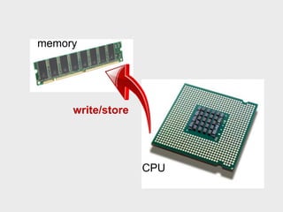
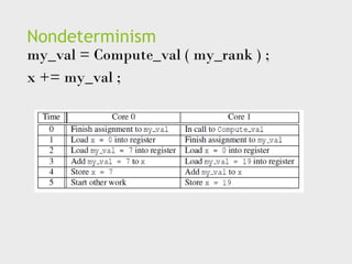
5. Main memory
 This is a collection of locations, each of which is
capable of storing both instructions and data.
 Every location consists of an address, which is used to
access the location, and the contents of the location.

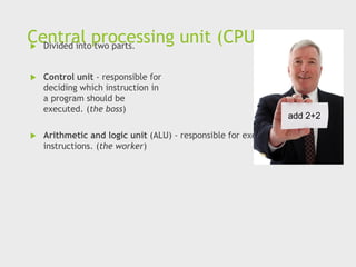
6. Central processing unit (CPU)
 Divided into two parts.
 Control unit - responsible for
deciding which instruction in
a program should be
executed. (the boss)
 Arithmetic and logic unit (ALU) - responsible for executing the actual
instructions. (the worker)
add 2+2

7. Key terms
 Register – very fast storage, part of the CPU.
 Program counter – stores address of the next
instruction to be executed.
 Bus – wires and hardware that connects the CPU and
memory.

8. memory
CPU
fetch/read

9. memory
CPU
write/store

10. von Neumann bottleneck

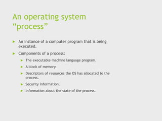
11. An operating system
“process”
 An instance of a computer program that is being
executed.
 Components of a process:
 The executable machine language program.
 A block of memory.
 Descriptors of resources the OS has allocated to the
process.
 Security information.
 Information about the state of the process.

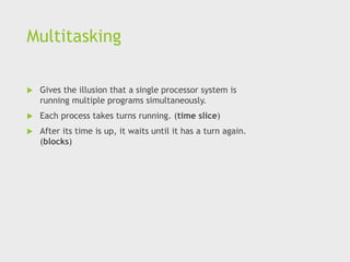
12. Multitasking
 Gives the illusion that a single processor system is
running multiple programs simultaneously.
 Each process takes turns running. (time slice)
 After its time is up, it waits until it has a turn again.
(blocks)

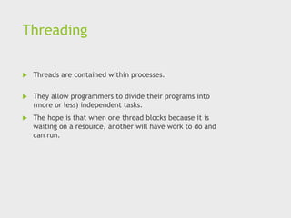
13. Threading
 Threads are contained within processes.
 They allow programmers to divide their programs into
(more or less) independent tasks.
 The hope is that when one thread blocks because it is
waiting on a resource, another will have work to do and
can run.

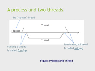
14. A process and two threads
Figure :Process and Thread
the “master” thread
starting a thread
Is called forking
terminating a thread
Is called joining

15. Modifications to the von
neumann model

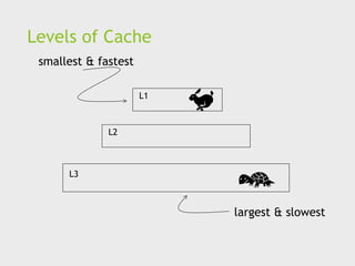
16. Basics of caching
 A collection of memory locations that can be accessed
in less time than some other memory locations.
 A CPU cache is typically located on the same chip, or
one that can be accessed much faster than ordinary
memory.

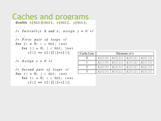
17. Principle of locality
 Accessing one location is followed by an access of a
nearby location.
 Spatial locality – accessing a nearby location.
 Temporal locality – accessing in the near future.

18. Principle of locality
float z[1000];
…
sum = 0.0;
for (i = 0; i < 1000; i++)
sum += z[i];

19. Levels of Cache
L1
L2
L3
smallest & fastest
largest & slowest

20. Cache hit
L1
L2
L3
x sum
y z total
A[ ] radius r1 center
fetch x

21. Cache miss
L1
L2
L3
y sum
r1 z total
A[ ] radius center
fetch x x
main
memory

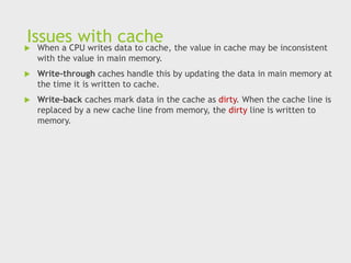
22. Issues with cache
 When a CPU writes data to cache, the value in cache may be inconsistent
with the value in main memory.
 Write-through caches handle this by updating the data in main memory at
the time it is written to cache.
 Write-back caches mark data in the cache as dirty. When the cache line is
replaced by a new cache line from memory, the dirty line is written to
memory.

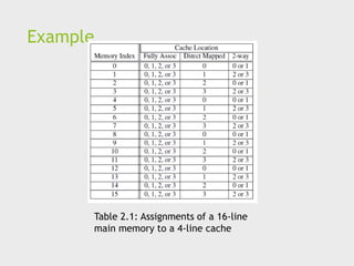
23. Cache mappings
 Full associative – a new line can be placed at any location in the cache.
 Direct mapped – each cache line has a unique location in the cache to
which it will be assigned.
 n-way set associative – each cache line can be place in one of n different
locations in the cache.

24. n-way set associative
 When more than one line in memory can be mapped to several
different locations in cache we also need to be able to decide which
line should be replaced or evicted.
x

25. Example
Table 2.1: Assignments of a 16-line
main memory to a 4-line cache

26. Caches and programs

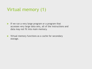
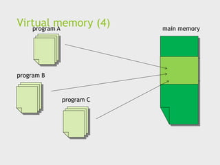
27. Virtual memory (1)
 If we run a very large program or a program that
accesses very large data sets, all of the instructions and
data may not fit into main memory.
 Virtual memory functions as a cache for secondary
storage.

28. Virtual memory (2)
 It exploits the principle of spatial and temporal locality.
 It only keeps the active parts of running programs in
main memory.

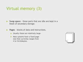
29. Virtual memory (3)
 Swap space - those parts that are idle are kept in a
block of secondary storage.
 Pages – blocks of data and instructions.
 Usually these are relatively large.
 Most systems have a fixed page
size that currently ranges from
4 to 16 kilobytes.

30. Virtual memory (4)
program A
program B
program C
main memory

31. Virtual page numbers
 When a program is compiled its pages are assigned
virtual page numbers.
 When the program is run, a table is created that maps
the virtual page numbers to physical addresses.
 A page table is used to translate the virtual address into
a physical address.

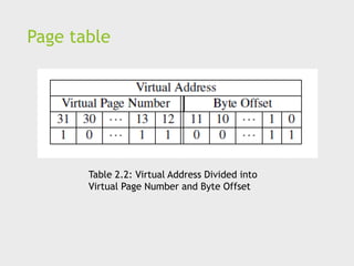
32. Page table
Table 2.2: Virtual Address Divided into
Virtual Page Number and Byte Offset

33.  Using a page table has the potential to significantly
increase each program’s overall run-time.
 A special address translation cache in the processor.

34. Translation-lookaside buffer (2)
 It caches a small number of entries (typically 16–512)
from the page table in very fast memory.
 Page fault – attempting to access a valid physical
address for a page in the page table but the page is only
stored on disk.

35.  Attempts to improve processor performance by having
multiple processor components or functional units
simultaneously executing instructions.

36. Instruction Level Parallelism (2)
 Pipelining - functional units are arranged in stages.
 Multiple issue - multiple instructions can be
simultaneously initiated.

37. Pipelining

38. Pipelining example (1)
Add the floating point numbers
9.87×104 and 6.54×103

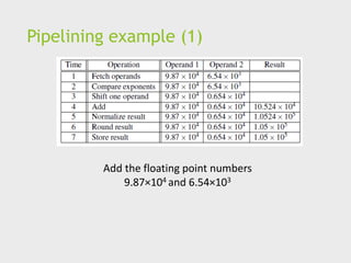
39. Pipelining example (2)
 Assume each operation
takes one nanosecond
(10-9 seconds).
 This for loop takes about
7000 nanoseconds.

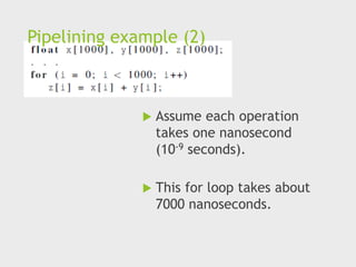
40. Pipelining (3)
 Divide the floating point adder into 7 separate pieces of
hardware or functional units.
 First unit fetches two operands, second unit compares
exponents, etc.
 Output of one functional unit is input to the next.

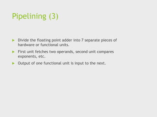
41. Pipelining (4)
Table 2.3: Pipelined Addition.
Numbers in the table are subscripts of operands/results.

42. Pipelining (5)
 One floating point addition still takes
7 nanoseconds.
 But 1000 floating point additions
now takes 1006 nanoseconds!

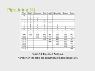
43. Multiple Issue (1)
 Multiple issue processors replicate functional units and try to
simultaneously execute different instructions in a program.
adder #1 adder #2
z[1]
z[3]
z[2]
z[4]
for (i = 0; i < 1000; i++)
z[i] = x[i] + y[i];

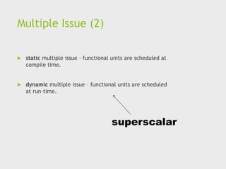
44. Multiple Issue (2)
 static multiple issue - functional units are scheduled at
compile time.
 dynamic multiple issue – functional units are scheduled
at run-time.
superscalar

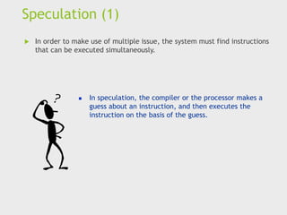
45. Speculation (1)
 In order to make use of multiple issue, the system must find instructions
that can be executed simultaneously.
◼ In speculation, the compiler or the processor makes a
guess about an instruction, and then executes the
instruction on the basis of the guess.

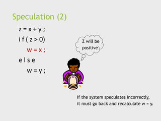
46. Speculation (2)
z = x + y ;
i f ( z > 0)
w = x ;
e l s e
w = y ;
Z will be
positive
If the system speculates incorrectly,
it must go back and recalculate w = y.

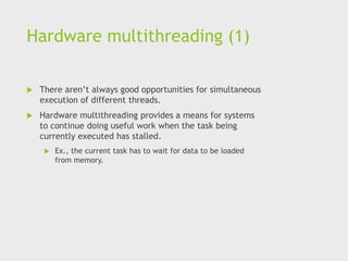
47. Hardware multithreading (1)
 There aren’t always good opportunities for simultaneous
execution of different threads.
 Hardware multithreading provides a means for systems
to continue doing useful work when the task being
currently executed has stalled.
 Ex., the current task has to wait for data to be loaded
from memory.

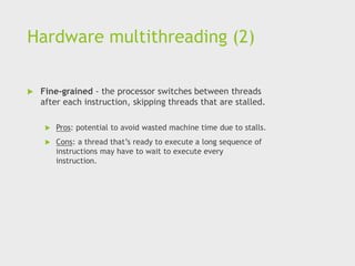
48. Hardware multithreading (2)
 Fine-grained - the processor switches between threads
after each instruction, skipping threads that are stalled.
 Pros: potential to avoid wasted machine time due to stalls.
 Cons: a thread that’s ready to execute a long sequence of
instructions may have to wait to execute every
instruction.

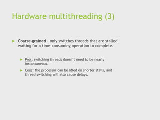
49. Hardware multithreading (3)
 Coarse-grained - only switches threads that are stalled
waiting for a time-consuming operation to complete.
 Pros: switching threads doesn’t need to be nearly
instantaneous.
 Cons: the processor can be idled on shorter stalls, and
thread switching will also cause delays.

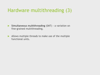
50. Hardware multithreading (3)
 Simultaneous multithreading (SMT) - a variation on
fine-grained multithreading.
 Allows multiple threads to make use of the multiple
functional units.

51. Parallel hardware
A programmer can write code to exploit.

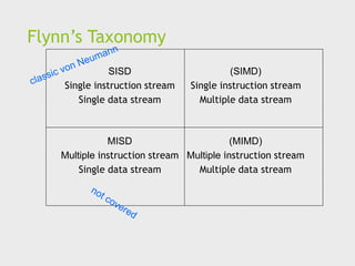
52. Flynn’s Taxonomy
SISD
Single instruction stream
Single data stream
(SIMD)
Single instruction stream
Multiple data stream
MISD
Multiple instruction stream
Single data stream
(MIMD)
Multiple instruction stream
Multiple data stream

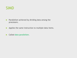
53. SIMD
 Parallelism achieved by dividing data among the
processors.
 Applies the same instruction to multiple data items.
 Called data parallelism.

54. SIMD example
control unit
ALU1 ALU2 ALUn
…
for (i = 0; i < n; i++)
x[i] += y[i];
x[1] x[2] x[n]
n data items
n ALUs

55. SIMD
 What if we don’t have as many ALUs as data items?
 Divide the work and process iteratively.
 Ex. m = 4 ALUs and n = 15 data items.
Round3 ALU1 ALU2 ALU3 ALU4
1 X[0] X[1] X[2] X[3]
2 X[4] X[5] X[6] X[7]
3 X[8] X[9] X[10] X[11]
4 X[12] X[13] X[14]

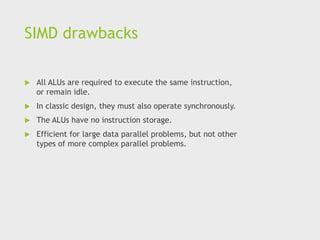
56. SIMD drawbacks
 All ALUs are required to execute the same instruction,
or remain idle.
 In classic design, they must also operate synchronously.
 The ALUs have no instruction storage.
 Efficient for large data parallel problems, but not other
types of more complex parallel problems.

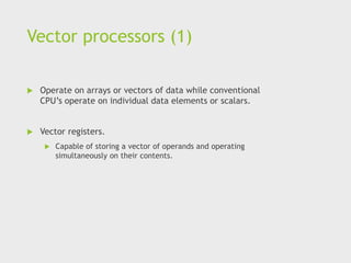
57. Vector processors (1)
 Operate on arrays or vectors of data while conventional
CPU’s operate on individual data elements or scalars.
 Vector registers.
 Capable of storing a vector of operands and operating
simultaneously on their contents.

58. Vector processors (2)
 Vectorized and pipelined functional units.
 The same operation is applied to each element in the
vector (or pairs of elements).
 Vector instructions.
 Operate on vectors rather than scalars.

59. Vector processors (3)
 Interleaved memory.
 Multiple “banks” of memory, which can be accessed more
or less independently.
 Distribute elements of a vector across multiple banks, so
reduce or eliminate delay in loading/storing successive
elements.
 Strided memory access and hardware scatter/gather.
 The program accesses elements of a vector located at
fixed intervals.

60. Vector processors - Pros
 Fast.
 Easy to use.
 Vectorizing compilers are good at identifying code to
exploit.
 Compilers also can provide information about code that
cannot be vectorized.
 Helps the programmer re-evaluate code.
 High memory bandwidth.
 Uses every item in a cache line.

61. Vector processors - Cons
 They don’t handle irregular
data structures as well as other
parallel architectures.
 A very finite limit to their ability to handle ever larger
problems. (scalability)

62. Graphics Processing Units
(GPU)
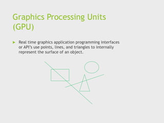
 Real time graphics application programming interfaces
or API’s use points, lines, and triangles to internally
represent the surface of an object.

63. GPUs
 A graphics processing pipeline converts the internal
representation into an array of pixels that can be sent
to a computer screen.
 Several stages of this pipeline
(called shader functions) are programmable.
 Typically just a few lines of C code.

64. GPUs
 Shader functions are also implicitly parallel, since they
can be applied to multiple elements in the graphics
stream.
 GPU’s can often optimize performance by using SIMD
parallelism.
 The current generation of GPU’s use SIMD parallelism.
 Although they are not pure SIMD systems.

65. MIMD
 Supports multiple simultaneous instruction streams
operating on multiple data streams.
 Typically consist of a collection of fully independent
processing units or cores, each of which has its own
control unit and its own ALU.

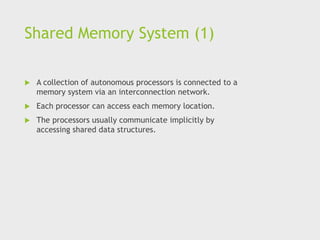
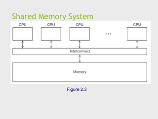
66. Shared Memory System (1)
 A collection of autonomous processors is connected to a
memory system via an interconnection network.
 Each processor can access each memory location.
 The processors usually communicate implicitly by
accessing shared data structures.

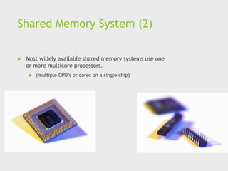
67. Shared Memory System (2)
 Most widely available shared memory systems use one
or more multicore processors.
 (multiple CPU’s or cores on a single chip)

68. Shared Memory System
Figure 2.3

69. UMA multicore system
Figure 2.5
Time to access all
the memory locations
will be the same for
all the cores.

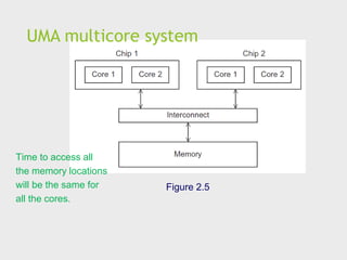
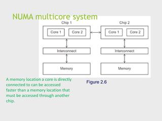
70. NUMA multicore system
Figure 2.6
A memory location a core is directly
connected to can be accessed
faster than a memory location that
must be accessed through another
chip.

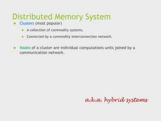
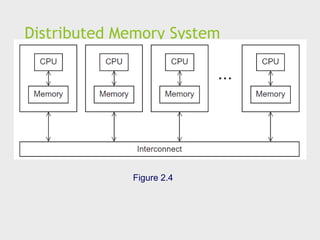
71. Distributed Memory System
 Clusters (most popular)
 A collection of commodity systems.
 Connected by a commodity interconnection network.
 Nodes of a cluster are individual computations units joined by a
communication network.
a.k.a. hybrid systems

72. Distributed Memory System
Figure 2.4

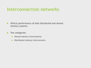
73. Interconnection networks
 Affects performance of both distributed and shared
memory systems.
 Two categories:
 Shared memory interconnects
 Distributed memory interconnects

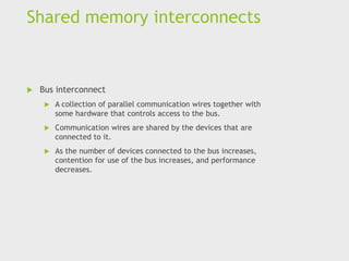
74. Shared memory interconnects
 Bus interconnect
 A collection of parallel communication wires together with
some hardware that controls access to the bus.
 Communication wires are shared by the devices that are
connected to it.
 As the number of devices connected to the bus increases,
contention for use of the bus increases, and performance
decreases.

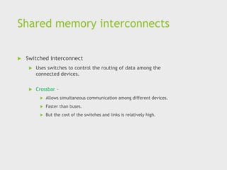
75. Shared memory interconnects
 Switched interconnect
 Uses switches to control the routing of data among the
connected devices.
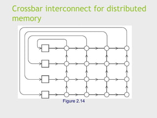
 Crossbar –
 Allows simultaneous communication among different devices.
 Faster than buses.
 But the cost of the switches and links is relatively high.

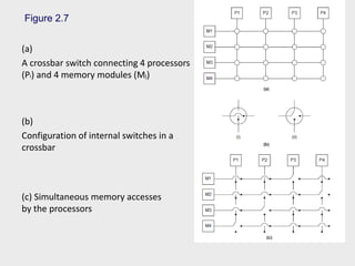
76. Figure 2.7
(a)
A crossbar switch connecting 4 processors
(Pi) and 4 memory modules (Mj)
(b)
Configuration of internal switches in a
crossbar
(c) Simultaneous memory accesses
by the processors

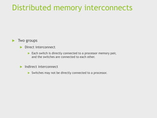
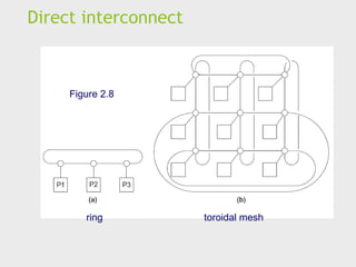
77. Distributed memory interconnects
 Two groups
 Direct interconnect
 Each switch is directly connected to a processor memory pair,
and the switches are connected to each other.
 Indirect interconnect
 Switches may not be directly connected to a processor.

78. Direct interconnect
Figure 2.8
ring toroidal mesh

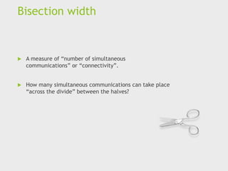
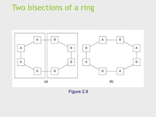
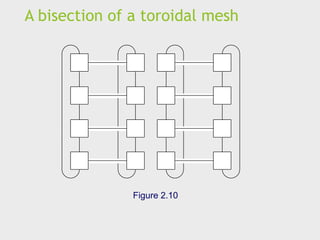
79. Bisection width
 A measure of “number of simultaneous
communications” or “connectivity”.
 How many simultaneous communications can take place
“across the divide” between the halves?

80. Two bisections of a ring
Figure 2.9

81. A bisection of a toroidal mesh
Figure 2.10

82. Definitions
 Bandwidth
 The rate at which a link can transmit data.
 Usually given in megabits or megabytes per second.
 Bisection bandwidth
 A measure of network quality.
 Instead of counting the number of links joining the halves,
it sums the bandwidth of the links.

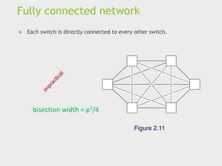
83. Fully connected network
 Each switch is directly connected to every other switch.
Figure 2.11
bisection width = p2/4

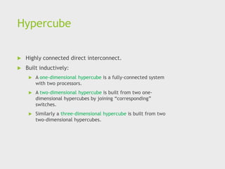
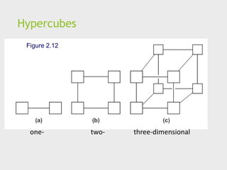
84. Hypercube
 Highly connected direct interconnect.
 Built inductively:
 A one-dimensional hypercube is a fully-connected system
with two processors.
 A two-dimensional hypercube is built from two one-
dimensional hypercubes by joining “corresponding”
switches.
 Similarly a three-dimensional hypercube is built from two
two-dimensional hypercubes.

85. Hypercubes
Figure 2.12
one- three-dimensional
two-

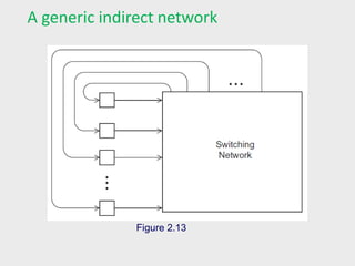
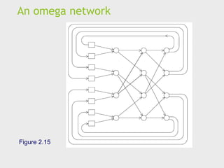
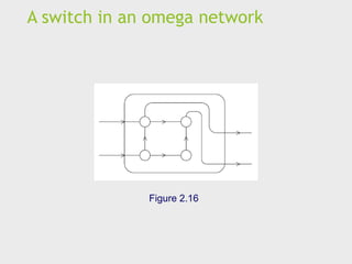
86. Indirect interconnects
 Simple examples of indirect networks:
 Crossbar
 Omega network
 Often shown with unidirectional links and a collection of
processors, each of which has an outgoing and an
incoming link, and a switching network.

87. A generic indirect network
Figure 2.13

88. Crossbar interconnect for distributed
memory
Figure 2.14

89. An omega network
Figure 2.15

90. A switch in an omega network
Figure 2.16

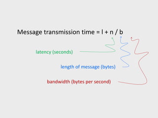
91. More definitions
 Any time data is transmitted, we’re interested in how long it will take for
the data to reach its destination.
 Latency
 The time that elapses between the source’s beginning to transmit the data and
the destination’s starting to receive the first byte.
 Bandwidth
 The rate at which the destination receives data after it has started to receive the
first byte.

92. Message transmission time = l + n / b
latency (seconds)
bandwidth (bytes per second)
length of message (bytes)

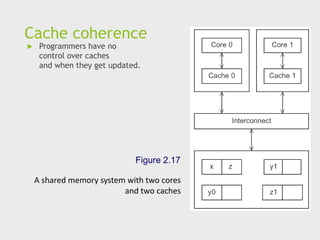
93. Cache coherence
 Programmers have no
control over caches
and when they get updated.
Figure 2.17
A shared memory system with two cores
and two caches

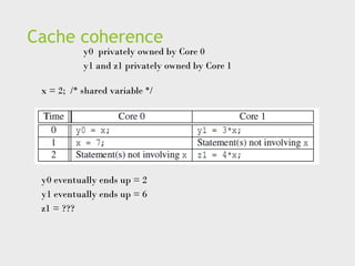
94. Cache coherence
x = 2; /* shared variable */
y0 privately owned by Core 0
y1 and z1 privately owned by Core 1
y0 eventually ends up = 2
y1 eventually ends up = 6
z1 = ???

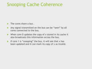
95. Snooping Cache Coherence
 The cores share a bus .
 Any signal transmitted on the bus can be “seen” by all
cores connected to the bus.
 When core 0 updates the copy of x stored in its cache it
also broadcasts this information across the bus.
 If core 1 is “snooping” the bus, it will see that x has
been updated and it can mark its copy of x as invalid.

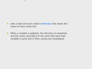
96.  Uses a data structure called a directory that stores the
status of each cache line.
 When a variable is updated, the directory is consulted,
and the cache controllers of the cores that have that
variable’s cache line in their caches are invalidated.

97. Parallel software

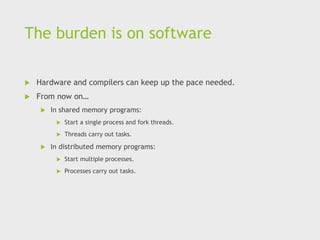
98. The burden is on software
 Hardware and compilers can keep up the pace needed.
 From now on…
 In shared memory programs:
 Start a single process and fork threads.
 Threads carry out tasks.
 In distributed memory programs:
 Start multiple processes.
 Processes carry out tasks.

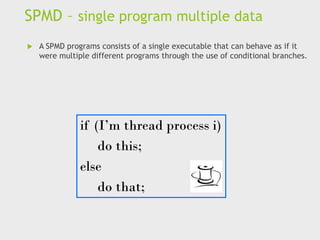
99. SPMD – single program multiple data
 A SPMD programs consists of a single executable that can behave as if it
were multiple different programs through the use of conditional branches.
if (I’m thread process i)
do this;
else
do that;

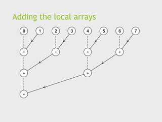
100. Writing Parallel Programs
double x[n], y[n];
…
for (i = 0; i < n; i++)
x[i] += y[i];
1. Divide the work among the
processes/threads
(a) so each process/thread
gets roughly the same
amount of work
(b) and communication is
minimized.
2. Arrange for the processes/threads to synchronize.
3. Arrange for communication among processes/threads.

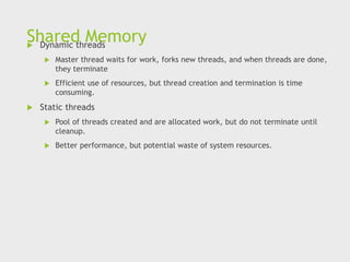
101. Shared Memory
 Dynamic threads
 Master thread waits for work, forks new threads, and when threads are done,
they terminate
 Efficient use of resources, but thread creation and termination is time
consuming.
 Static threads
 Pool of threads created and are allocated work, but do not terminate until
cleanup.
 Better performance, but potential waste of system resources.

102. Nondeterminism
. . .
printf ( "Thread %d > my_val = %dn" ,
my_rank , my_x ) ;
. . .
Thread 0 > my_val = 7
Thread 1 > my_val = 19
Thread 1 > my_val = 19
Thread 0 > my_val = 7

103. Nondeterminism
my_val = Compute_val ( my_rank ) ;
x += my_val ;

104. Nondeterminism
 Race condition
 Critical section
 Mutually exclusive
 Mutual exclusion lock (mutex, or simply lock)
my_val = Compute_val ( my_rank ) ;
Lock(&add_my_val_lock ) ;
x += my_val ;
Unlock(&add_my_val_lock ) ;

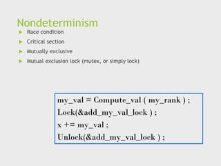
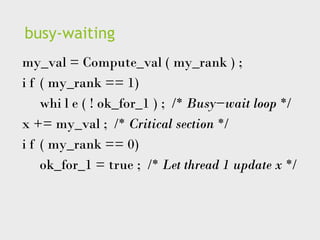
105. busy-waiting
my_val = Compute_val ( my_rank ) ;
i f ( my_rank == 1)
whi l e ( ! ok_for_1 ) ; /* Busy−wait loop */
x += my_val ; /* Critical section */
i f ( my_rank == 0)
ok_for_1 = true ; /* Let thread 1 update x */

106. message-passing
char message [ 1 0 0 ] ;
. . .
my_rank = Get_rank ( ) ;
i f ( my_rank == 1) {
sprintf ( message , "Greetings from process 1" ) ;
Send ( message , MSG_CHAR , 100 , 0 ) ;
} e l s e i f ( my_rank == 0) {
Receive ( message , MSG_CHAR , 100 , 1 ) ;
printf ( "Process 0 > Received: %sn" , message ) ;
}

107. Partitioned Global Address Space
Languages
shared i n t n = . . . ;
shared double x [ n ] , y [ n ] ;
private i n t i , my_first_element , my_last_element ;
my_first_element = . . . ;
my_last_element = . . . ;
/ * Initialize x and y */
. . .
f o r ( i = my_first_element ; i <= my_last_element ; i++)
x [ i ] += y [ i ] ;

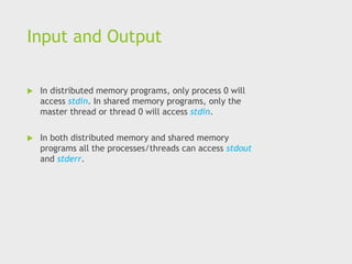
108. Input and Output
 In distributed memory programs, only process 0 will
access stdin. In shared memory programs, only the
master thread or thread 0 will access stdin.
 In both distributed memory and shared memory
programs all the processes/threads can access stdout
and stderr.

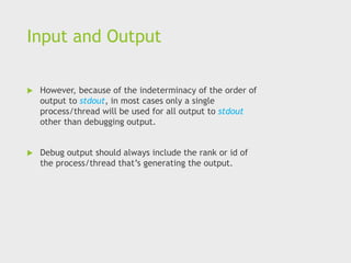
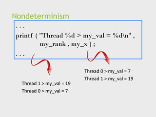
109. Input and Output
 However, because of the indeterminacy of the order of
output to stdout, in most cases only a single
process/thread will be used for all output to stdout
other than debugging output.
 Debug output should always include the rank or id of
the process/thread that’s generating the output.

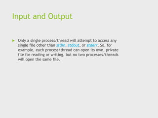
110. Input and Output
 Only a single process/thread will attempt to access any
single file other than stdin, stdout, or stderr. So, for
example, each process/thread can open its own, private
file for reading or writing, but no two processes/threads
will open the same file.

111. Performance

112. Speedup
 Number of cores = p
 Serial run-time = Tserial
 Parallel run-time = Tparallel
Tparallel = Tserial / p

113. Speedup of a parallel
program
Tserial
Tparallel
S =

114. Efficiency of a parallel
program
E =
Tserial
Tparallel
S
p
=
p
=
Tserial
p Tparallel
.

115. Speedups and efficiencies of a parallel
program

116. Speedups and efficiencies of parallel
program on different problem sizes

117. Speedup

118. Efficiency

119. Effect of overhead
Tparallel = Tserial / p + Toverhead

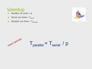
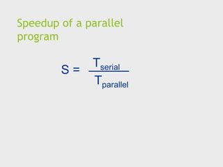
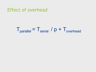
120. Amdahl’s Law
 Unless virtually all of a serial program is parallelized,
the possible speedup is going to be very limited —
regardless of the number of cores available.

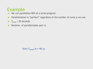
121. Example
 We can parallelize 90% of a serial program.
 Parallelization is “perfect” regardless of the number of cores p we use.
 Tserial = 20 seconds
 Runtime of parallelizable part is
0.9 x Tserial / p = 18 / p

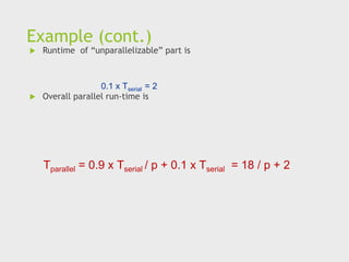
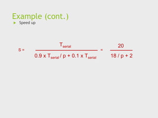
122. Example (cont.)
 Runtime of “unparallelizable” part is
 Overall parallel run-time is
0.1 x Tserial = 2
Tparallel = 0.9 x Tserial / p + 0.1 x Tserial = 18 / p + 2

123. Example (cont.)
 Speed up
0.9 x Tserial / p + 0.1 x Tserial
Tserial
S = =
18 / p + 2
20

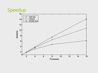
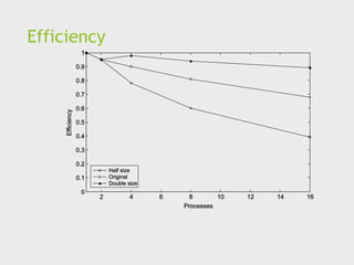
124. Scalability
 In general, a problem is scalable if it can handle
ever increasing problem sizes.
 If we increase the number of processes/threads
and keep the efficiency fixed without increasing
problem size, the problem is strongly scalable.
 If we keep the efficiency fixed by increasing the
problem size at the same rate as we increase
the number of processes/threads, the problem
is weakly scalable.

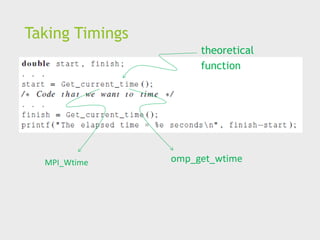
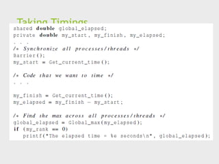
125. Taking Timings
 What is time?
 Start to finish?
 A program segment of interest?
 CPU time?
 Wall clock time?

126. Taking Timings
theoretical
function
MPI_Wtime omp_get_wtime

127. Taking Timings

128. Taking Timings

129. Parallel program
design

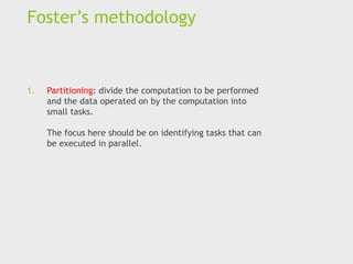
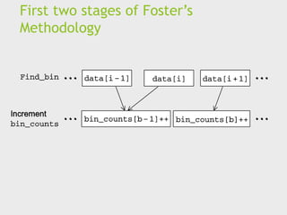
130. Foster’s methodology
1. Partitioning: divide the computation to be performed
and the data operated on by the computation into
small tasks.
The focus here should be on identifying tasks that can
be executed in parallel.

131. Foster’s methodology
2. Communication: determine what communication
needs to be carried out among the tasks identified in
the previous step.

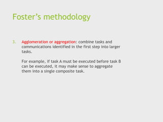
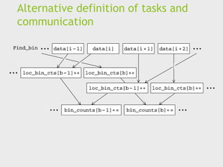
132. Foster’s methodology
3. Agglomeration or aggregation: combine tasks and
communications identified in the first step into larger
tasks.
For example, if task A must be executed before task B
can be executed, it may make sense to aggregate
them into a single composite task.

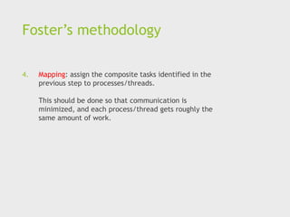
133. Foster’s methodology
4. Mapping: assign the composite tasks identified in the
previous step to processes/threads.
This should be done so that communication is
minimized, and each process/thread gets roughly the
same amount of work.

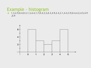
134. Example - histogram
 1.3,2.9,0.4,0.3,1.3,4.4,1.7,0.4,3.2,0.3,4.9,2.4,3.1,4.4,3.9,0.4,4.2,4.5,4.9
,0.9

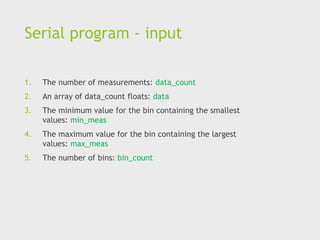
135. Serial program - input
1. The number of measurements: data_count
2. An array of data_count floats: data
3. The minimum value for the bin containing the smallest
values: min_meas
4. The maximum value for the bin containing the largest
values: max_meas
5. The number of bins: bin_count

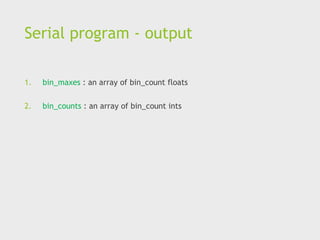
136. Serial program - output
1. bin_maxes : an array of bin_count floats
2. bin_counts : an array of bin_count ints

137. First two stages of Foster’s
Methodology

138. Alternative definition of tasks and
communication

139. Adding the local arrays

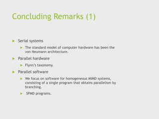
140. Concluding Remarks (1)
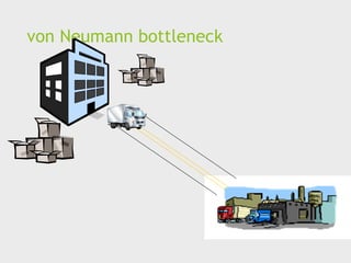
 Serial systems
 The standard model of computer hardware has been the
von Neumann architecture.
 Parallel hardware
 Flynn’s taxonomy.
 Parallel software
 We focus on software for homogeneous MIMD systems,
consisting of a single program that obtains parallelism by
branching.
 SPMD programs.

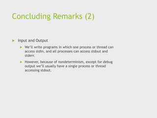
141. Concluding Remarks (2)
 Input and Output
 We’ll write programs in which one process or thread can
access stdin, and all processes can access stdout and
stderr.
 However, because of nondeterminism, except for debug
output we’ll usually have a single process or thread
accessing stdout.

142. Concluding Remarks (3)
 Performance
 Speedup
 Efficiency
 Amdahl’s law
 Scalability
 Parallel Program Design
 Foster’s methodology

143. References
1. Peter S Pacheco, Matthew
Malensek – An Introduction to
Parallel Programming, second
edition, Morgan Kauffman.