A study of himreen reservoir water quality using in situ
GSA poster
1. Kelly Devlin*, Paul Zarella, Ashley Newman, Jonathan Nyquist, and Laura Toran
Department of Earth and Environmental Science, Temple University, Philadelphia, PA 19122, kellydevlin@temple.edu*
Introduction
Wells and Monitoring
Experiment
References
.
Acknowledgements
References
Conclusion
Temple University recently constructed its Science Education and Research (SERC)
between existing Engineering building and Gladfelter Hall. The building is LEED Gold
certified, and has incorporated many structures and techniques including drainage
pipes to prevent excess stormwater runoff. Members of the Department of Earth and
Environmental Science (EES) drilled wells in the infiltration basin located behind the
building during its construction. The lined basin contains 15 drainage pipes
surrounded by gravel and topped off with replaced fill, also known as urban soil. The
wells were used to monitor the effectiveness of this basin over time. SERC was
designed to have a reduced environmental impact and monitoring will determine if it
is meeting its purpose.
Figure 1:
LiDAR scan
of infiltration
basin
Figure 2: Schematic of drainage pipes in basin
Figure 3: Map view of the study
area on Temple University’s main
campus, showing the extent of the
vegetated infiltration basin and well
locations. This basin is designed to
cover a 9000 sq. ft. area and has a
5:1 impervious area to infiltration
area ratio.
Figure 4: Groundwater hydrograph after basin completion
and cistern tie in.
Three wells were drilled in the basin in three separate locations. We calculated
approximate layers based on the well data and basin schematic available to us. These
wells showed uneven recharge in the water table, as seen in Figure 4, though they are
placed within approximately 12 to 20 m of each other. One proposed reason was uneven
infiltration within the basin, which we decided to test. Ground-penetrating radar (GPR) has
been shown to be effective in measuring soil moisture content (Lunt et. al., 2005; Jadoon
et. al., 2012), so we used this technique along with soil moisture sensors and a LiDAR
scan.
Figure 5: Cross-
Section view of the
infiltration basin.
Direct infiltration at
the surface is
contributing
stormwater inflow.
1. I. Lunt, S. Hubbard, Y. Rubin, Soil moisture content estimation using
ground-penetrating radar reflection data, Journal of Hydrology 307, 254-
269 (2005).
2. K.Z. Jadoon et. al., Estimation of soil hydraulic parameters in the field by
integrated hydrogeophysical inversion of time-lapse ground-penetrating
radar data, Vadose Zone Journal 11 (2012).
3. Project Tracking Number: 2011-TEMP-1739-01, PWD stromwater
descriptions (2011).
4. McClymont and Rak Geotechnical Engineers LLC, Project No.4266,
Geotechnical Investigation Report (2011).
Funding was provided by the EPA STAR Grant, the Science Scholars
Program, and the Undergraduate Research Program. Additional thanks to the
members of the Department of Earth and Environmental Science and Temple
University Facilities Management for help completing this project.
• A 15 m by 5 m grid was laid out over the basin in order to create 3D
GPR surveys.
• Two sprinklers were allowed to water the grid for two hours.
• Five surveys were conducted using a Mala Pro-Ex System and 800 MHz
antenna, one before the induced rain event, one immediately after the
event, and three
during the recovery period.
• Five Decagon capacitance sensors collected soil moisture data starting
both before and after the event.
• A Trimble TX-5 terrain-based LiDAR system performed a 3D scan of the
basin to collect topographic data in a separate survey
Figure 6 (left) showing Mala Pro-Ex System and Figure 7
(right) showing data collection using GPR system.
Figure 10: The volumetric water
content (VWC) of the five sensors
plotted over the recovery period.
Uneven infiltration rates could be
seen, with Sensor 5 suggesting it was
not yet in a recovery period by the
end of the surveys.
Figures 8 and 9: A digital elevation
map (DEM) obtained by the LiDAR
unit and derived Total Wetness Index
(TWI) map. GPR scans shown in
Figures 11 and 12 are marked with
red lines. The grid has low
topography with a slight incline going
downhill in the –x direction. This
offers some insight to the infiltration
patterns seen with the GPR. In
Figure 11, Sensor 5 is shown to have
a lower TWI than the other sensors,
possibly explaining its VWC over
time.
Figure 10: GPR radargrams at the 4.25 m mark of the grid,
closest to SERC. Radargrams are in order from top to bottom:
baseline (dry), immediately after sprinklers were turned off
(wet), and three sequential recovery periods. The urban soil
causes a high attenuation rate in all surveys, leading to little
penetration below 8 ns. Structure of interest shown within red
rectangles with a .
Two-wayTraveltime(ns)
Distance (m)
Signal is lost
around 8 ns,
or about 2 m
• The GPR scans did not contain structures that resembled the
water table, failing to provide more groundwater data.
• This was due to high clay content in the top layer of urban
soil and the resulting attenuation. Infiltration and changes in
soil moisture were seen with the GPR, further showing this
technique is useful in mapping soil moisture.
• The capacitance sensors showed uneven recovery rates
among themselves. This can be explained by the LiDAR
data, which shows slight topographic relief within the grid.
• Further tests to be conducted in the basin include
infiltrometer and slug tests to gather data on the hydraulic
conductivity at this site.
Figure 11: Radargrams from Figure 10 are zoomed in within red rectangles
to show structures. A structure can be seen between 3.5 m and 4.5 m,
denoted by red dot. As the soil becomes wet and dries, the structure loses
and regains definition. The banding can also be seen with a delay of
approximately .75 ns with the wetter surveys. The delay is caused by
increased water content which reduces the radar wave velocity.
GPR Results
Distance (m)
Two-wayTraveltime(ns)
Distance (m)
Two-wayTraveltime(ns)
Figure 12: Radargrams from an alternative scan within the grid created,
located at the 1.5 m mark. The scans have been formatted on a scale
comparable to Figure 11. Unlike the previous scans, a distinct structure
cannot be seen. A tangible difference between subsequent scans after
wetting is difficult to observe. This can be attributed to different
subsurface structures as well as uneven infiltration.
Editor's Notes
Copyright Colin Purrington (http://colinpurrington.com/tips/academic/posterdesign).