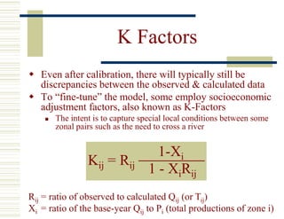
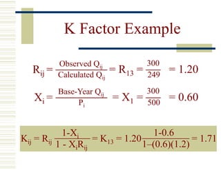
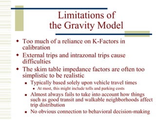
The document discusses the gravity model for trip distribution in transportation planning. It describes the key variables and equations in the gravity model, including productions, attractions, friction factors, and impedances. It also covers applying the gravity model through calibration, using an iterative process to determine the calibration constant c and compare modeled vs observed trip distributions. Socioeconomic adjustment factors (K-factors) can be used to further refine model fits but have limitations. The gravity model has limitations as well, such as overreliance on K-factors and simplistic impedance factors.

1. Advanced
Transportation Engineering
The Four-Step Model:
II. Trip Distribution

2. The
Gravity
Model

3. The Gravity Model
The bigger the friction factor,
the more trips that are encouraged
Tij = Qij =
Pi Aj FijKij
ΣAzFizKi
j
Fij = 1 / Wc
ij
(Productions)(Attractions)(Friction Factor)
Sum of the (Attractions x Friction Factors) of the Zones
=
= Pipij
& ln F = - c ln W

4. Some of the Variables
Tij = Qij = Trips Volume between i & j
Fij =1/Wc
ij = Friction Factor
Wij = Generalized Cost (including travel time, cost)
c = Calibration Constant
pij = Probability that trip i will be attracted to zone j
kij = Socioeconomic Adjustment Factor

5. To Apply the Gravity Model
What we need…
1. Productions, {Pi}
2. Attractions, {Aj}
3. Skim Tables {Wij)
 Target-Year Interzonal Impedances

6. Gravity Model Example 8.2
 Given:
 Target-year Productions, {Pi}
 Relative Attractiveness of Zones, {Aj}
 Skim Table, {Wij}
 Calibration Factor, c = 2.0
 Socioeconomic Adjustment Factor, K = 1.0
 Find:
 Trip Interchanges, {Qij}

7. Attractions vs. Attractiveness
 The number of attractions to a particular zone
depends upon the zone’s attractiveness
 As compared to the attractiveness of all the other
competing zones and
 The distance between them
 Two zones with identical attractiveness may
have a different number of attractions due to one’s
remote location
 Thus, substituting attractions for attractiveness
can lead to incorrect results

8. Σ(AzFizKij)
Calculate Friction Factors, {Fij}
TAZ Productions
1 1500
2 0
3 2600
4 0
Σ 4100
TAZ "Attractiveness"
1 0
2 3
3 2
4 5
Σ 10
TAZ 1 2 3 4
1 5 10 15 20
2 10 5 10 15
3 15 10 5 10
4 20 15 10 5
Calibration Factor
c = 2.0
Socioeconomic Adj. Factor
K = 1.0
TAZ 1 2 3 4
1 0.0400 0.0100 0.0044 0.0025
2 0.0100 0.0400 0.0100 0.0044
3 0.0044 0.0100 0.0400 0.0100
4 0.0025 0.0044 0.0100 0.0400
TAZ 1 2 3 4 Σ
1 0.0000 0.0300 0.0089 0.0125 0.0514
2 0.0000 0.1200 0.0200 0.0222 0.1622
3 0.0000 0.0300 0.0800 0.0500 0.1600
4 0.0000 0.0133 0.0200 0.2000 0.2333
TAZ 1 2 3 4
1 0.0000 0.5838 0.1730 0.2432
2 0.0000 0.7397 0.1233 0.1370
3 0.0000 0.1875 0.5000 0.3125
4 0.0000 0.0571 0.0857 0.8571
TAZ 1 2 3 4 Σ
1 0 876 259 365 1500
2 0 0 0 0 0
3 0 488 1300 813 2600
4 0 0 0 0 0
Σ 0 1363 1559 1177 4100
Target-Year Inter-zonal
Impedances, {Wij}
F11=
1
52 = 0.04
AjFijKij=A4F34K34= (5)(0.01)(1.0)
= 0.05
Given…
Find Denominator of Gravity Model Equation {AjFijKij}
Find Probability that Trip i will be attracted to Zone j, {pij}
Find Trip Interchanges, {Qij}
pij =
AjFijKij
0.16
=
0.05
= 0.3125
Qij = Pipij = (2600)(0.3125) = 813
Fij =
1
Wc
ij
=

9. Keep in mind that the socioeconomic
factor, K, can be a matrix of value
rather than just one value
TAZ 1 2 3 4
1 1.4 1.2 1.7 1.9
2 1.2 1.1 1.1 1.4
3 1.7 1.1 1.5 1.3
4 1.9 1.4 1.3 1.6

10. Calibration of
the Gravity Model
 When we talk about calibrating the
gravity model, we are referring to
determining the numerical value c
 The reason we do this is to fix the
relationship between the travel-time
factor and the inter-zonal impedance

11. Calibration of
the Gravity Model
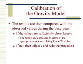
 Calibration is an iterative process
 We first assume a value of c and then use:
Qij = Pi
Aj Fij
Σ(Ax Fix)
[ ]
Qij = Tij = Trips Volume between i & j
Fij =1 / Wc
ij = Friction Factor
Wij = Generalized Cost (including travel time, cost)
c = Calibration Constant

12. Calibration of
the Gravity Model
 The results are then compared with the
observed values during the base year
 If the values are sufficiently close, keep c
 The results are expressed in terms of the
appropriate equation relating F and W with c
 If not, then adjust c and redo the procedure

13. Trip-Length Frequency Distribution
 Compares the observed and computed
Qij values

14. Gravity Model
Calibration Example
Given:
Zone 2
Zone 3
Zone 4
Zone 5
Zone 1
5 TAZ City
TAZ Productions
1 500
2 1000
3 0
4 0
5 0
Σ 1500
TAZ "Attractiveness"
1 0
2 0
3 2
4 3
5 5
Σ 10
TAZ 3 4 5
1 5 10 15
2 10 5 15
Target-Year Inter-zonal Impedances, {Wij}
5
5
10
10
15
15
Find: c and Kij to fit the base data
TAZ 3 4 5
1 300 150 50
2 180 600 220
Base-Year Trip Interchange Volumes, {tij}

15. Relating F & W
 Starting with:
 Take the natural log of both sides
 Now c is the slope of a straight
line relating ln F and ln W
Fij =
1
Wc
ij
ln F = - c ln W
ln
F
ln W

16. Trip-Length Frequency Distribution
 Group zone pairs by max Wij
 Sum Interchange Volumes for each set of zone pairs
 Find f = (Σtix) / (Σtij)
TAZ 3 4 5
1 5 10 15
2 10 5 15
Target-Year Inter-zonal Impedances, {Wij}
TAZ 3 4 5
1 300 150 50
2 180 600 220
Base-Year Trip Interchange Volumes, {tij}
W Σtij f
5 300 600 900 0.60
10 150 180 330 0.22
15 50 220 270 0.18
Σ 1500 1.00
tij Values
Zone Pairs
13, 24
14, 23
15, 25

17. Let’s assume c = 2.0
TAZ 3 4 5
1 5 10 15
2 10 5 15
Target-Year Inter-zonal
Impedances, {Wij} Base-Year Trip Interchange Volumes, {tij}
First Iteration
TAZ 3 4 5 Σ
1 300 150 50 500
2 180 600 220 1000
Friction Factor, {Fij} with c = 2.0
TAZ 3 4 5
1 0.040 0.010 0.004
2 0.010 0.040 0.004
Fij =
1
Wc
ij
= F13=
1
52 = 0.04

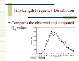
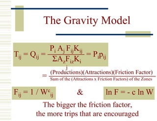
18. c = 2.0
First Iteration
Aj Fij
TAZ 3 4 5 Σ
1 0.605 0.227 0.168 1.000
2 0.123 0.740 0.137 1.000
TAZ 3 4 5 Σ
1 0.080 0.030 0.022 0.132
2 0.020 0.120 0.022 0.162
Aj Fij
Σ(Ax Fix)
[ ]
TAZ "Attractiveness"
1 0
2 0
3 2
4 3
5 5
Σ 10
Friction Factor, {Fij} with c = 2.0
TAZ 3 4 5
1 0.040 0.010 0.004
2 0.010 0.040 0.004

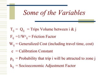
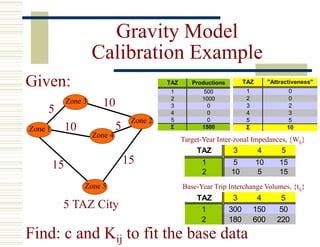
19. c = 2.0
First Iteration
TAZ 3 4 5 Σ
1 0.605 0.227 0.168 1.000
2 0.123 0.740 0.137 1.000
TAZ 3 4 5 Σ
1 303 113 84 500
2 123 740 137 1000
W Σtij f
5 303 740 1042.2 0.69
10 113 123 236.73 0.16
15 84 137 221.02 0.15
Σ
1 5 0 0 1 . 0 0
15, 25
Zone Pairs tij Values
13, 24
14, 23
Aj Fij
Σ(Ax Fix)
[ ]
Qij = Pi
Aj Fij
Σ(Ax Fix)
[ ]
TAZ Productions
1 500
2 1000
3 0
4 0
5 0
Σ 1500

20. Trip-Length FrequencyDistribution
0
0.1
0.2
0.3
0.4
0.5
0.6
0.7
0.8
0.9
1
5 10 15
Base Year Iteration 2 (c=1.5)

21. Let’s assume c = 1.5
TAZ 3 4 5
1 5 10 15
2 10 5 15
Target-Year Inter-zonal
Impedances, {Wij} Base-Year Trip Interchange Volumes, {tij}
Second Iteration
TAZ 3 4 5 Σ
1 300 150 50 500
2 180 600 220 1000
Friction Factor, {Fij} with c = 1.5
Fij =
1
Wc
ij
= F13=
1
51.5 = 0.089
TAZ 3 4 5
1 0.089 0.032 0.017
2 0.032 0.089 0.017

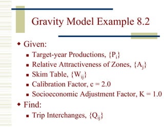
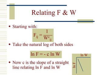
22. c = 1.5
Second Iteration
Aj Fij
Aj Fij
Σ(Ax Fix)
[ ]
TAZ "Attractiveness"
1 0
2 0
3 2
4 3
5 5
Σ 10
Friction Factor, {Fij} with c = 1.5
TAZ 3 4 5
1 0.089 0.032 0.017
2 0.032 0.089 0.017
TAZ 3 4 5 Σ
1 0.179 0.095 0.086 0.360
2 0.063 0.268 0.086 0.418
TAZ 3 4 5 Σ
1 0.497 0.264 0.239 1.000
2 0.151 0.642 0.206 1.000

23. c = 1.5
Second Iteration
Aj Fij
Σ(Ax Fix)
[ ]
Qij = Pi
Aj Fij
Σ(Ax Fix)
[ ]
TAZ Productions
1 500
2 1000
3 0
4 0
5 0
Σ 1500
TAZ 3 4 5 Σ
1 0.497 0.264 0.239 1.000
2 0.151 0.642 0.206 1.000
TAZ 3 4 5 Σ
1 249 132 120 500
2 151 642 206 1000
W Σtij f
5 249 642 891.06 0.59
10 132 151 283.26 0.19
15 120 206 325.67 0.22
Σ
1 5 0 0 1 . 0 0
Zone Pairs tij Values
13, 24
14, 23
15, 25

24. Trip-Length FrequencyDistribution
0
0.1
0.2
0.3
0.4
0.5
0.6
0.7
0.8
0.9
1
5 10 15
Base Year Iteration 1 (c=2.0) Iteration 2 (c=1.5)

25. K Factors
 Even after calibration, there will typically still be
discrepancies between the observed & calculated data
 To “fine-tune” the model, some employ socioeconomic
adjustment factors, also known as K-Factors
 The intent is to capture special local conditions between some
zonal pairs such as the need to cross a river
Kij = Rij
1-Xi
1 - XiRij
Rij = ratio of observed to calculated Qij (or Tij)
Xi = ratio of the base-year Qij to Pi (total productions of zone i)

26. K Factor Example
Rij =
Observed Qij
Calculated Qij
= R13 =
300
249
= 1.20
Xi =
Base-Year Qij
Pi
= X1 =
300
500
= 0.60
Kij = Rij
1-Xi
1 - XiRij
= K13 = 1.20
1-0.6
1–(0.6)(1.2)
= 1.71

27. The Problem with K-Factors
 Although K-Factors may improve the model
in the base year, they assume that these
special conditions will carry over to future
years and scenarios
 This limits model sensitivity and undermines the
model’s ability to predict future travel behavior
 The need for K-factors often is a symptom
of other model problems.
 Additionally, the use of K-factors makes it more
difficult to figure out the real problems

28. Limitations of
the Gravity Model
 Too much of a reliance on K-Factors in
calibration
 External trips and intrazonal trips cause
difficulties
 The skim table impedance factors are often too
simplistic to be realistic
 Typically based solely upon vehicle travel times
 At most, this might include tolls and parking costs
 Almost always fails to take into account how things
such as good transit and walkable neighborhoods affect
trip distribution
 No obvious connection to behavioral decision-making