The document outlines various laboratory experiments in geotechnical engineering, focusing on soil property assessment through both visual inspection and standard testing methods. The objectives include determining soil properties such as specific gravity, liquid limit, plastic limit, and conducting unconfined compression tests. Detailed procedures and data tables for sample collection and analysis are provided to facilitate accurate soil classification and evaluation.

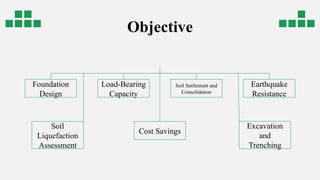
1. 0. Geotechnical Engineering Lab

2. 02
.
03
.
04
.
05
.
Conclusions
Sample collection
Experiments
Analysis
01
.
Introduction
Objective
Table of contents
06
.

3. Sample Collection

4. Introduction
Geotechnical Engineering is the specialty of Civil Engineering which deals
with the property and behavior of soil and rock in engineering purposes. To
obtain different properties of soil, laboratory tests are performed on collected
disturbed and undisturbed soil samples, while field tests are performed on
sub-soil at in-situ condition following mainly standard ASTM methods.

5. Objective
Earthquake
Resistance
Soil Settlement and
Consolidation
Load-Bearing
Capacity
Foundation
Design
Soil
Liquefaction
Assessment
Cost Savings
Excavation
and
Trenching

6. Field Identification of soil
The objective of the experiment is
make a rapid assessment of soil
without the aid of apparatus also
identify and describe the soil by
visual manual procedure.

7. Procedure:
1) Identify the color (e.g. brown, gray, brownish gray), odor (if any) and texture
(coarse or fine-grained) of soil.
2) Identify the major soil constituent (¿50% by weight) using Table 2.1 as coarse
gravel, fine gravel, coarse sand, medium sand, fine sand, or fines.
3) If the major soil constituent is sand or gravel:
a) Identify particle distribution
b) Identify particle shape (angular, sub-angular, rounded, sub-
rounded) using.
4) If the major soil constituents are fines, perform the following tests:
a) Dry strength test
b) Dilatancy test
c) Plasticity (or Toughness) test
5) Identify moisture condition (dry, moist, wet or saturated)
6) Record visual classification of the soil.

8. Data table
Name of test Observation Probable soil type Moisture condition Identified soil type
Dry strength High to very high Clay
Dry Dry clay
Dilatancy None Clay
Organic Clay
Plasticity
(Toughness)
Tough Clay
Dispersion Several hours to
days
Clay
Organic Clay

9. Specefic Gravity
of Soil

10. Equipment
• Pycnometer (volumetric bottle)
• Balance
• Manometer
• Heat source
• Drying oven
• Desiccator
• Thermometer (graduated to 0.1 ◦ C)
• Evaporating dishes

11. Procedure
• Put approximately 150 gm of oven dry soil, weighed to 0.01 gm into a calibrated
pycnometer which is already half full of deaired, distilled water. Be sure that no soil grains
are lost when they are put into the pycnometer.
• Remove all of the air which is entrapped in the soil by 10 minutes of boiling. Accompany
the boiling with continuous agitation.
• Cool the bottle and suspension to some temperature within the range of the calibration
curve for the bottle.
• Add water to bring the bottom of the meniscus to the calibration mark.
• Dry the outside of the bottle and the inside of the neck above the meniscus.
• Weigh the bottle with water and soil in it to 0.01 gm.

12. Data Sheet
Specefic Gravity of Soil
Experimental
Weight of clean dry pycnometer (gm) 109.8
Weight of pycnometer + water + soil,M1(gm) 435.96
Temperatutre , T( 25
Weight of pycnometer + water, M2 (gm) 359
Dry weight of soil, Ms (gm) 129.5
Specific gravity of water at T, GT 0.9971
Specific gravity of soil, Gs 2.45

13. Sample Calculation
Weight of pycnometer = 109.8 gm
Weight of pycnometer + Dry soil = 238.9 gm
Weight of dry soil = 129.5 gm
Weight of pycnometer + soil + water = 435.96 gm
Weight of pycnometer + water = 359 gm
Temperature = 25
Specefic gravity of water at T,GT =0.9971
Specefic Gravity of soil,Gs = (MsGT)/(MS-M1+M2)
= (129.5 x 0.9971)/(129.5-435.96+359)
= 2.45

14. Grain Size Analysis
by Hydrometer

15. Equipment
• 152H Hydrometer
• Sedimentation cylinder
• Control cylinder
• Thermometer
• Beaker
• Timing device

16. Procedure
• Place 50 g of fine soil in a beaker and
add dispersing agent.
• While the soil is soaking, add 125 mL
of the dispersing agent to the control
cylinder and fill it to the mark with
distilled water.
• Record zero and meniscus correction
• Insert the hydrometer and
thermometer into the control cylinder.
• Take hydrometer readings after elapsed time
of 1, 2, 5, 10, 15, 30, 60 minutes and 24
hours.

17. Data Sheet
Sieve Analysis
Sieve number Sieve
opening
(mm)
Materials
retained (gm)
% of
Materials
retained
Cumulative %
retained
% finer
#4 4.75 0 0 0 100
#8 2.36 0 0 0 100
#16 1.18 0 0 0 100
#30 0.60 0 0 0 100
#50 0.30 5 2.5 2.5 97.5
#100 0.15 60 30 32.5 67.5
#200 0.075 25 12.5 45 55
Pan - 110 55 100 -
Total=200 FM=0.35

18. Sieve Analysis
Graph

19. Data Sheet
Date Time T
(min)
Temp
,
Ractual Rm L
(mm)
D
(min) CT a Rc P PA
25-
Sept
11:06
AM
0 25 34 34 107 - - - - - -
25-
Sept
11:07
AM
1 25 30 30 114 0.04
59
1.3 1.06 27.3 57.
9
31.8
25-
Sept
11:08
AM
2 25 26 26 120 0.03
33
1.3 1.06 23.3 49.
4
27.1
25-
Sept
11:11
AM
5 25 22 22 127 0.02
17
1.3 1.06 19.3 40.
9
22.5
25-
Sept
11:16
AM
10 25 19 19 132 0.01
56
1.3 1.06 16.3 34.
6
19.03
25-
Sept
11:21
AM
15 25 18 18 133 0.01
28
1.3 1.06 15.3 32.
4
17.8
25-
Sept
11:36
AM
30 25 17 17 135 0.00
91
1.3 1.06 14.3 30.
3
16.7
25-
Sept
12:0
6 PM
60 25 16 16 137 0.00
65
1.3 1.06 13.3 28.
2
15.5
26-
Sept
11:06
PM
1440 25 13 13 142 0.00
14
1.3 1.06 10.3 21.
8
12
Hydrometer number : 152H
Specefic gravity of soil : 2.457
Dispersing agent : Sodium
Hexamet-
aphosphate
Weight of soil sample : 50 gm
Zero correction : 4
Meniscus correction : 0

20. Sample Calculation
Zero correction = +4
Meniscus correction = +0
For t = 1 min,
Actual hydrometer reading, Ractual = 30
Meniscus corrected reading, Rm = 30 + 0 = 30
Effective hydrometer depth for Rm = 30 (from Table 4.1), L = 114 mm
Specific gravity of soil, Gs = 2.45
Viscosity of water at 25◦ C, µ = 8.95 milli poise = 0.000895 Ns/m2
Equivalent particle diameter,
D x

21. Sample Calculation
=0.0459 mm
Temperature correction factor (from Table 4.2), CT = +1.30
Specific gravity correction factor (from Table 4.3), a = 1.06
Corrected hydrometer reading, Rc = Ractual − zero correction + CT = 30 − 4 + 1.3 = 27.3
Percent finer,
P =
=
=57.9
Adjusted percent finer,
PA =
=
= 31.8

22. Hydrometer Analysis
Graph
0.001 0.01 0.1
0
10
20
30
40
50
60
70
Hydrometer analysic distribution curve
Particle Size
%Fine

23. Combined
Graph
0.001 0.01 0.1 1 10
0
10
20
30
40
50
60
70
80
90
100
110
Hydrometer and Sieve analysic combination graph
Particle size
%Fine

24. Determination of
Liquid Limit

25. Equipmen
t
• Liquid Limit Device (Casangrande Apparatus)
• Grooving Tool
• #40 Sieve
• Porcelain (Evaporating) dish
• Moisture Cans
• Balance
• Desiccator
• Glass plate
• Spatula
• Wash bottle filled with distilled water
• Drying Oven

26. Procedure
• Take about 100 gm of moist soil and mix it
thoroughly with distilled water to form a uniform
paste.
• In the liquid limit device cup, cut a groove at
the center of the soil paste using the
standard grooving tool.
• Lift the cup and drop it from a height of 12
mm using the crank-operated cam.
• Record the moisture content from the soil
taken from the connected point.

27. Data Sheet
Sample
No.
No.of
blows,N
Moistur
e
Can No.
Wt. of
can
(gm)
Wt. of
can
+wet
soil
(gm)
Wt. of
can +
dry soil
(gm)
Wt. of
Dry soil
(gm)
Wt. of
water
(gm)
Water
content
w (%)
1 15 LL-30 15.37 48.71 40.35 24.98 8.36 33.47
2 22 LL-40 13.76 36.76 31.52 17.49 5.24 29.96
3 38 LL-F 21.86 60.50 51.99 33.13 8.51 25.69
4 24 LL-B 11.35 42.92 35.74 24.39 7.18 29.44
5 19 LL-G 22.73 60.27 51.57 28.84 8.7 30.17

28. Sample Calculation
For moisture can no. LL-30
Weight of can = 15.37 gm
Wt. of can + wet soil = 48.71 gm
Wt. of can + dry soil = 40.35 gm
Wt. of dry soil = Wt. of can + dry soil – Wt. of can
=(40.35 – 15.37)= 24.98 gm
Wt. of water=Wt of can + wet soil – Wt. of can + dry soil
=( 48.71 – 40.35)= 8.36 gm
Moisture content= = 33.47 %

29. Liquid Limit Graph

30. Plastic Limit
The Plastic Limit (PL) is the moisture content at which a fine-grained
soil can no longer be remolded without cracking.

31. • Conduct the plastic limit experiment.
• Identify the plastic limit value for soil.
• Identify the importance and application of plastic
limit test.
To determine the plastic
limit of soil
01 Objective
LEARNING OUTCOME
02

32. Apparatus
Glass plate
Moisture
Cans
Drying Oven

33. Procedu
re
• Mix thoroughly he soil sample with water.
• Roll the soil on a glass plate with the
hand until it is reached to 3.2 mm (1/8
inch) in diameter.
• Take some of the crumbling soil obtained
for water content determination.
• Determine the water content of the
sample.

34. Data Table
Sample No
Moisture
Can no
Mass of can
(gm)
Mass of can
+ Wet soil
(gm)
Mass of can
+ Dry soil
(gm)
Mass of
Dry soil
(gm)
Mass of
Water (gm)
Water
Content
(%) P
Average
water
content (%),
PL
1 PL-M 5.95 10.74 9.91 3.96 0.83 20.959596
21.04517
2 PL-A 6.46 11.69 10.78 4.32 0.91 21.064815
3 PL-50 11.59 17.04 16.09 4.5 0.95 21.111111

35. Shrinkage Limit
the water content at which the soil changes from a semi-solid to a
solid state

36. • Identify the shrinkage limit value for soil
• Identify the importance and application of plastic
limit test.
To determine the
shrinkage limit of soil
01 Objective
NEED AND SCOPE
02

37. Apparatus
Shrinkage
DISK
Mercury Balance

38. Procedu
re
 Determine the weight of Dish.
 Use a knife to remove the excess soil standing
above the edge of the dish and to level it.
 Weigh the dish containing wet soil.
 Keep the dish with wet soil in dry oven for 24
hours.
 Cool the soil and weigh dish with dry soil.
 Place a small dish in a larger one and fill the small
one to overflow with mercury.
 Immerse the oven dry sample in mercury and
weigh the mercury that is displaced by the dry soil
pat.

39. Data Table
Mass of dish (gm) 56.29
Mass of dish + wet soil (gm) 82.20
Mass of dish + dry soil (gm) 74.82
Mass of dry soil (gm) 18.53
Mass water (gm) 7.38
Mass of displaced Mercury (gm) 142
Volume of dry soil (cm3
) 10.48
Shrinkage limit, SL (%) 15.97

40. Unconfined
compression
Test
One of the fastest and
cheapest methods of
measuring shear strength of
clayey soil.

41. design and stability analysis of foundations,
retaining walls, slopes, and embankments
To determine the Unconfiend
compression strength (qu) of
cohesive soil
01 Objective
Practical
Application
02

42. Apparatus
Unconfined
compression device
Load and
deformation dial
gauges
Sample trimming
equipment

43. Procedu
re
 Extrude the soil sample from Shelby tube
sampler.
 Measure the exact diameter of the top of the
specimen
 Weigh the sample and record the mass on the
data sheet
 Calculate the deformation (∆L)
corresponding to 15% strain
 Keep applying the load until the load (load
dial) decreases on the specimen significantly

44. Data Table
Deforma
tion dial
readin
load dial
reading
Sample
deformation(mm)
Initial Specimen
Height
(mm)
Strain
ϵ
% Strain
Cross Sectional
Area,
(m
2
)
Corrected Area,
(m
2
)
Load,
(KN)
Stress, (KPa)
0 0.00 0.00 80.56 0.00000 0.00000 0.00131 0.00131 -0.09550 0.00000
50 2.00 0.50 80.56 0.00621 0.62066 0.00131 0.00132 -0.07350 0.00000
100 4.00 1.00 80.56 0.01241 1.24131 0.00131 0.00133 -0.05150 0.00000
150 6.00 1.50 80.56 0.01862 1.86197 0.00131 0.00134 -0.02950 0.00000
200 7.50 2.00 80.56 0.02483 2.48262 0.00131 0.00135 -0.01300 0.00000
250 9.00 2.50 80.56 0.03103 3.10328 0.00131 0.00135 0.00350 2.58383
300 10.30 3.00 80.56 0.03724 3.72393 0.00131 0.00136 0.01780 13.05647
350 11.50 3.50 80.56 0.04345 4.34459 0.00131 0.00137 0.03100 22.59221
400 12.50 4.00 80.56 0.04965 4.96524 0.00131 0.00138 0.04200 30.41020
450 13.60 4.50 80.56 0.05586 5.58590 0.00131 0.00139 0.05410 38.91541
500 14.40 5.00 80.56 0.06207 6.20655 0.00131 0.00140 0.06290 44.94802
550 15.00 5.50 80.56 0.06827 6.82721 0.00131 0.00141 0.06950 49.33571
600 15.90 6.00 80.56 0.07448 7.44786 0.00131 0.00142 0.07940 55.98793
650 16.20 6.50 80.56 0.08069 8.06852 0.00131 0.00143 0.08270 57.92382
700 16.50 7.00 80.56 0.08689 8.68918 0.00131 0.00144 0.08600 59.82851
750 16.50 7.50 80.56 0.09310 9.30983 0.00131 0.00145 0.08600 59.42184
800 16.50 8.00 80.56 0.09930 9.93049 0.00131 0.00146 0.08600 59.01518
850 16.20 8.50 80.56 0.10551 10.55114 0.00131 0.00147 0.08270 56.35958
900 15.50 9.00 80.56 0.11172 11.17180 0.00131 0.00148 0.07500 50.75743

45. Graph

46. Graph (c0ntinued)

47. Direct shear
Test
Experimental procedure
conducted in geotechnical
engineering practice and
research that aims to
determine the shear strength
of soil materials.

48.  Assessing the stability of slopes or
cuts
 Finding the bearing capacity of
foundations
 Determining the earth pressure
exerted by a soil on a retaining wall.
To determine the direct shear strength of soil
materials
01 Objective
Practical
Application
02

49. Apparatus
Direct shear device
Load and deformation
dial gauges
Proving ring

50. Procedu
re
 Measure the diameter and height of the shear box.
 Place the sand into the shear box and level off the
top
 Set the vertical load (or pressure) to a
predetermined value
 Start the motor with selected speed so that the rate
of shearing is at a selected constant rate
 Continue taking readings until the horizontal shear
load peaks and then falls, or the horizontal
displacement reaches 15% of the diameter.

51. Data Table

52. Data Table (c0ntinued)

53. Graph

54. Graph (c0ntinued)

55. Result & Discussion

56. Test Results
Tests Results
Field Identification of soil Dry Clay
Specific Gravity 2.45
Sieve Analysis
Sandy Clay Soil (No direct gradation
based on Cu & Cc)
Atterberg Limits
LL=27.5% , PL= 21.05% , SL=15.97%,
PI=6.45%
If=3.30% , IT=1.95
Unconfined Compression Test qu =60 kPa , cu = 30 kPa
Deirect Shear Test Φ=29.05° , c = 0 kPa

57. Clay
Bearing Capacity
No heavy structures!
Dispersion
Less Erosion
Dilatancy
Difficulty in
Embankment
Construction
Plasticity
Better Interlocking

58. Organic Soil
Specific Gravity Range : 1.00 – 2.60

59. Low
Plasticity
LL<50%
Organic Clay
55% passes No. 200
Sieve
4<PI<7 , Above ‘A’ line
Sandy
100% Passing no. 4
sieve,45% retained on
no. 200
Fine Soil
Sandy Organic Clay

60. Swelling
Potential
Soil
Compactio
n
Atterberg Limits
SL>15%
Moisture Content
Liquid Limit
Plastic Limit

61. Organic Clay
Medium Consistency
Remolded Sample
Cu
qu
Error
Medium Consistency

62. Organic Clay
Direct Shear test
● In slope stability
● Error!

63. Conclusion

64. Organic Clay
Not Suitable For Footing Construction

65. Possible Solutions
Ground Improvement
Pile Foundation
Deeper strata with high bearing
capacity
Dynamic Compaction
Grouting