Download to read offline


![The idea that increased weathering rates
associated with tectonic uplift increases erosion
and removes enough carbon dioxide from the
atmosphere to control climate has its dissenters.
Ollier (2004a) identified what he termed ‘three
misconceptions’ in the relationships between
erosion, weathering, and carbon dioxide. First,
weathering and erosion are not necessarily cur-
rent processes – erosion, especially erosion in
mountainous regions, may occur with little
chemical alteration of rock or mineral fragments.
Second, in most situations, hydrolysis and not
carbonation is the chief weathering process –
weathering produces clays and not carbonates.
Furthermore, evidence suggests that chemical
weathering rates have declined since the mid- or
early Tertiary, before which time deep weathering
profiles formed in broad plains. Today, deep
weathering profiles form only in the humid
tropics. Third, Ollier questions the accepted
chronology of mountain building, which sees
Tibet, the highlands of western North America,
and the Andes beginning to rise about 40 million
years ago, favouring instead rise over the last few
million years.
HUMANS AS GEOMORPHIC
AGENTS
Geomorphic footprint
Over the last two centuries or so, humans have had
an increasingly significant impact on the transfer
of Earth materials and the modification of
landforms, chiefly through agricultural practices,
mining and quarrying, and the building of roads
and cities. As Harrison Brown (1956, 1031)
commented:
A population of 30 billion would consume rock
at a rate of about 1,500 tons per year. If we were
to assume that all the land areas of the world
were available for such processing, then, on
the average, man [sic] would “eat” his way
downward at a rate of 3.3 millimeters per year,
or over 3 meters per millennium. This figure
gives us some idea of the denudation rates that
might be approached in the centuries ahead.
And it gives us an idea of the powers for
denudation which lie in mankind’s hands.
The ‘geomorphic footprint’ is a measure of the
rate at which humans create new landforms and
mobilize sediment (Rivas et al. 2006). For four
study areas – one in northern Spain and three in
central and eastern Argentina – new landforms
were created by excavation and mining activities
at a rate of 7.9 m2
per person per year in the
Spanish area and 5.93 m2
per person per year in
the Argentinean areas. The volume of sediment
created by these activities was 30.4 m3
per person
per year and 6.4 m3
per person per year for the
Spanish and Argentinean areas respectively. These
values convert to a sediment mobilization rate of
2.4 mm/yr for the Spanish study site and 0.8
mm/yr for the Argentinian study sites, which
values exceed the rate mobilization of sediment by
natural processes by an order of magnitude of
two. If these figures are typical of other human-
dominated areas, then Brown’s denudation rates
may be reached during the present century with
a smaller population.
Humans have become increasingly adept at
ploughing land and at excavating and moving
materials in construction and mining activities.
Indeed, humans are so efficient at unintentionally
and deliberately moving soils and sediments that
they have become the leading geomorphic agent
of erosion (e.g. Hooke 2000). Placing human-
induced erosion in a geological perspective
demonstrates the point (Wilkinson 2005). The
weathered debris stored in continental and oceanic
sedimentary rocks suggest that, on average,
continental surfaces have lowered through natural
denudation at a rate of a few tens of metres per
million years. By contrast, construction, mining,
and agricultural activities presently transport
sediment and rock, and lower all ice-free
continental surfaces by a few hundred metres per
million years. Therefore, the human species is
80 INTRODUCING LANDFORMS AND LANDSCAPES](https://image.slidesharecdn.com/fundamentalsofgeomorphologyroutledgefundamentalsofphysicalgeography-220921044803-9a19de6c/85/fundamentalsofgeomorphology_routledgefundamentalsofphysicalgeography-pdf-97-320.jpg)


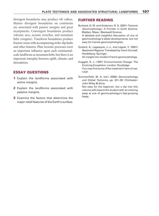


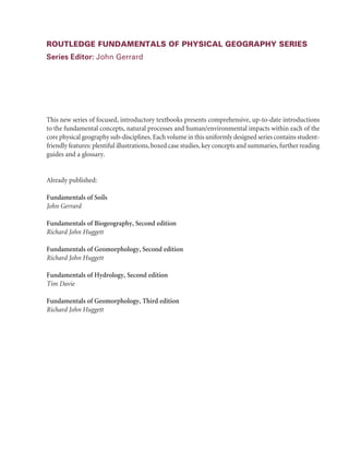
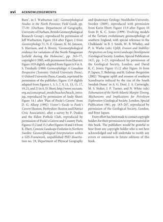
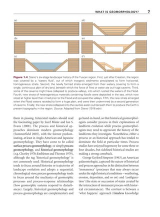
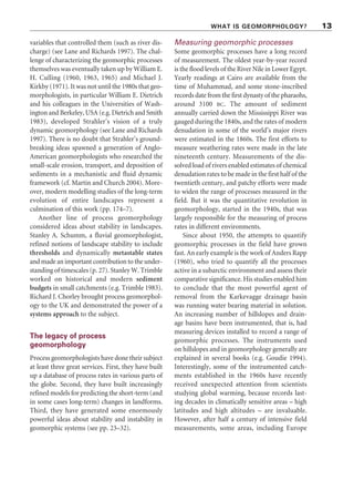
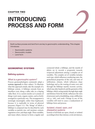
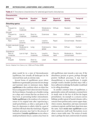
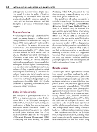
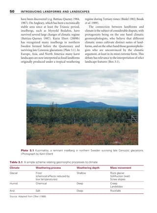
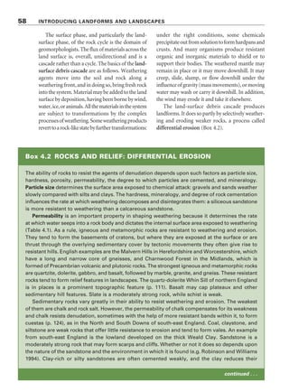
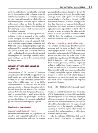
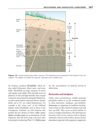
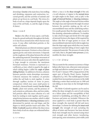
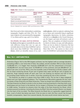
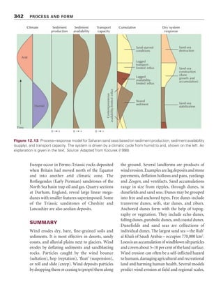
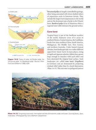
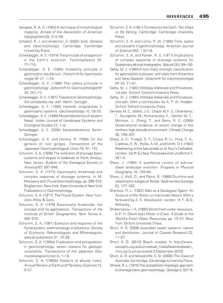
![WEATHERING AND ASSOCIATED LANDFORMS 143
pH is a measure of the acidity or alkalinity of aqueous solutions. The term stands for the
concentration of hydrogen ions in a solution, with the p standing for Potenz (the German
word for ‘power’). It is expressed as a logarithmic scale of numbers ranging from about 0 to 14
(Figure 7.2). Formulaically, pH = –log[H+
], where [H+
] is the hydrogen ion concentration (in gram-
equivalents per litre) in an aqueous solution. A pH of 14 corresponds to a hydrogen ion con-
centration of 10–14
gram-equivalents per
litre. A pH of 7, which is neutral (neither
acid nor alkaline), corresponds to a
hydrogen ion concentration of 10–7
gram-
equivalents per litre. A pH of 0 corresponds
to a hydrogen ion concentration of 10–0
(= 1) gram-equivalents per litre. A solution
with a pH greater than 7 is said to be
alkaline, whereas a solution with a pH
less than 7 is said to be acidic (Figure 7.2).
In weathering, any precipitation with a
pH below 5.6 is deemed to be acidic and
referred to as ‘acid rain’.
The solubility of minerals also depends
upon the Eh or redox (reduction–oxida-
tion) potential of a solution. The redox
potential measures the oxidizing or
reducing characteristics of a solution. More
specifically, it measures the ability of a
solution to supply electrons to an oxidizing
agent, or to take up electrons from a
reducing agent. So redox potentials are
electrical potentials or voltages. Solutions
may have positive or negative redox
potentials, with values ranging from about
–0.6 volts to +1.4 volts. High Eh values
correspond to oxidizing conditions, while
low Eh values correspond to reducing
conditions.
Combined, pH and Eh determine the
solubility of clay minerals and other
weathering products. For example,
goethite, a hydrous iron oxide, forms
where Eh is relatively high and pH is
medium. Under high oxidizing conditions
(Eh +100 millivolts) and a moderate pH,
it slowly changes to hematite.
Box 7.2 pH AND Eh
Figure 7.2 The pH scale, with the pH of assorted
substances shown.](https://image.slidesharecdn.com/fundamentalsofgeomorphologyroutledgefundamentalsofphysicalgeography-220921044803-9a19de6c/85/fundamentalsofgeomorphology_routledgefundamentalsofphysicalgeography-pdf-160-320.jpg)
![Hydration
Hydration is transitional between chemical and
mechanical weathering. It occurs when minerals
absorbwatermoleculesontheiredgesandsurfaces,
or, for simple salts, in their crystal lattices, without
otherwise changing the chemical composition of
the original material. For instance, if water is added
to anhydrite, which is calcium sulphate (CaSO4),
gypsum(CaSO4.2H2O)isproduced.Thewaterinthe
crystal lattice leads to an increase of volume, which
maycausehydrationfoldingingypsumsandwiched
between other beds. Under humid mid-latitude
climates, brownish to yellowish soil colours are
caused by the hydration of the reddish iron oxide
hematitetorust-colouredgoethite.Thetakingupof
water by clay particles is also a form of hydration. It
leads to the clay’s swelling when wet. Hydration
assists other weathering processes by placing water
molecules deep inside crystal structures.
Oxidation and reduction
Oxidation occurs when an atom or an ion loses an
electron,increasingitspositivechargeordecreasing
its negative charge. It involves oxygen combining
with a substance. Oxygen dissolved in water is a
prevalent oxidizing agent in the environment.
Oxidation weathering chiefly affects minerals
containing iron, though such elements as
manganese, sulphur, and titanium may also be
oxidized.Thereactionforiron,whichoccursmainly
whenoxygendissolvedinwatercomesintocontact
with iron-containing minerals, is written:
4Fe2 + 3O2 + 2e → 2Fe2O3 [e = electron]
Alternatively, the ferrous iron, Fe2+
, which
occurs in most rock-forming minerals, may be
converted to its ferric form, Fe3+
, upsetting the
neutral charge of the crystal lattice, sometimes
causing it to collapse and making the mineral
more prone to chemical attack.
If soil or rock becomes saturated with stagnant
water, it becomes oxygen-deficient and, with the
aid of anaerobic bacteria, reduction occurs.
Reduction is the opposite of oxidation, and the
changes it promotes are called gleying. In colour,
gley soil horizons are commonly a shade of
grey.
The propensity for oxidation or reduction to
occur is shown by the redox potential, Eh. This is
measured in units of millivolts (mV), positive
values registering as oxidizing potential and
negative values as reducing potential (Box 7.2).
Carbonation
Carbonation is the formation of carbonates, which
are the salts of carbonic acid (H2CO3). Carbon
dioxidedissolvesinnaturalwaterstoformcarbonic
acid. The reversible reaction combines water with
carbon dioxide to form carbonic acid, which then
dissociatesintoahydrogenionandabicarbonateion.
Carbonicacidattacksminerals,formingcarbonates.
Carbonationdominatestheweatheringofcalcareous
rocks (limestones and dolomites) where the main
mineral is calcite or calcium carbonate (CaCO3).
Calcite reacts with carbonic acid to form calcium
hydrogencarbonate(Ca(HCO3)2)that,unlikecalcite,
is readily dissolved in water. This is why some
limestones are so prone to solution (p. 393). The
reversible reactions between carbon dioxide, water,
and calcium carbonate are complex. In essence, the
process may be written:
CaCO3 + H2O + CO2 ⇔ Ca2+
+ 2HCO3
–
This formula summarizes a sequence of events
starting with dissolved carbon dioxide (from the
air) reacting speedily with water to produce
carbonic acid, which is always in an ionic state:
CO2 + H2O ⇔ H+
+ HCO3
Carbonate ions from the dissolved limestone react
at once with the hydrogen ions to produce
bicarbonate ions:
CO3
2–
+ H+
⇔ HCO3
2–
This reaction upsets the chemical equilibrium in
the system, more limestone goes into solution to
144 PROCESS AND FORM](https://image.slidesharecdn.com/fundamentalsofgeomorphologyroutledgefundamentalsofphysicalgeography-220921044803-9a19de6c/85/fundamentalsofgeomorphology_routledgefundamentalsofphysicalgeography-pdf-161-320.jpg)


![The natural vegetation of the Southern Great Plains of Colorado, Kansas, New Mexico,
Oklahoma, and Texas is prairie grassland that is adapted to low rainfall and occasional
severe droughts. During the ‘Dirty Thirties’, North American settlers arrived from the
east. Being accustomed to more rainfall, they ploughed up the prairie and planted wheat.
Wet years saw good harvests; dry years, which were common during the 1930s, brought
crop failures and dust storms. In 1934 and 1935, conditions were atrocious. Livestock
died from eating excessive amounts of sand, human sickness increased because of the
dust-laden air. Machinery was ruined, cars were damaged, and some roads became
impassable. A report of the time evokes the starkness of the conditions:
The conditions around innumerable farmsteads are pathetic. A common farm scene
is one with high drifts filling yards, banked high against buildings, and partly or
wholly covering farm machinery, wood piles, tanks, troughs, shrubs, and young trees.
In the fields near by may be seen the stretches of hard, bare, unproductive subsoil
and sand drifts piled along fence rows, across farm roads, and around Russian-
thistles and other plants. The effects of the black blizzards [massive dust storms that
blotted out the Sun and turned day into night] are generally similar to those of snow
blizzards. The scenes are dismal to the passerby; to the resident they are demoralizing.
(Joel 1937, 2)
The results were the abandonment of farms and an exodus of families, remedied only
when the prairies affected were put back under grass. The effects of the dust storms
were not always localized:
On 9 May [1934], brown earth from Montana and Wyoming swirled up from the
ground, was captured by extremely high-level winds, and was blown eastward toward
the Dakotas. More dirt was sucked into the airstream, until 350 million tons were riding
toward urban America. By late afternoon the storm had reached Dubuque and
Madison, and by evening 12 million tons of dust were falling like snow over Chicago
– 4 pounds for each person in the city. Midday at Buffalo on 10 May was darkened
by dust, and the advancing gloom stretched south from there over several states,
moving as fast as 100 miles an hour. The dawn of 11 May found the dust settling over
Boston, New York, Washington, and Atlanta, and then the storm moved out to sea.
Savannah’s skies were hazy all day 12 May; it was the last city to report dust conditions.
But there were still ships in the Atlantic, some of them 300 miles off the coast, that
found dust on their decks during the next day or two.
(Worster 1979, 13–14)
Box 12.2 THE DUST BOWL
AEOLIAN LANDSCAPES 337](https://image.slidesharecdn.com/fundamentalsofgeomorphologyroutledgefundamentalsofphysicalgeography-220921044803-9a19de6c/85/fundamentalsofgeomorphology_routledgefundamentalsofphysicalgeography-pdf-356-320.jpg)


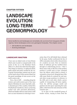

![LANDSCAPE INACTION
I have seen no inland rocks in Great Britain
which seem to point so unequivocally to the
action of the sea as the Brimham Rocks
[Plate 15.1], about nine miles from Harrogate.
They fringe an eminence, or upheaved island,
partly spared and partly wrecked by the sea.
A group of picturesque columns may be seen
on the eastern shore of this ancient island, but
the grand assemblage of ruins occurs on the
north-western side . . .
First, a line of cliff . . . extending along the
western and north-western part of the risen
island of Brimham for more than half a mile.
A detached part of this coastline, behind Mrs
Weatherhead’s farmhouse, shows a projecting
arched rock with associated phenomena,
which one familiar with sea-coast scenery could
have no more hesitation in referring to wave-
action than if he still beheld them whitened
by the spray. Farther northwards the line of
cliff in some places shows other characteristics
of a modern sea-coast. Here an immense
block of millstone grit has tumbled down
through an undermining process – there a
block seems ready to fall, but in that perilous
position it would seem to have remained
since the billows which failed to detach it
retreated to a lower level. Along the base of the
cliffs many blocks lie scattered far and near,
and often occupy positions in reference to
the cliffs and to each other which a power
capable of transporting will alone explain.
From the cliff-line passages ramify and
graduate into the spaces separating the rocky
pillars, which form the main attraction of this
romantic spot. . . .
As we gaze on this wonderful group of
insular wrecks, varying in form from the
CHAPTER FIFTEEN
LANDSCAPE
EVOLUTION:
LONG-TERM
GEOMORPHOLOGY
15
Some landforms and landscapes are remarkably old, survivors from long-gone climatic
regimes. Some landscapes evolve over geological timescales. This chapter covers:
• Old landforms and landscapes
• Evolving landscapes](https://image.slidesharecdn.com/fundamentalsofgeomorphologyroutledgefundamentalsofphysicalgeography-220921044803-9a19de6c/85/fundamentalsofgeomorphology_routledgefundamentalsofphysicalgeography-pdf-452-320.jpg)


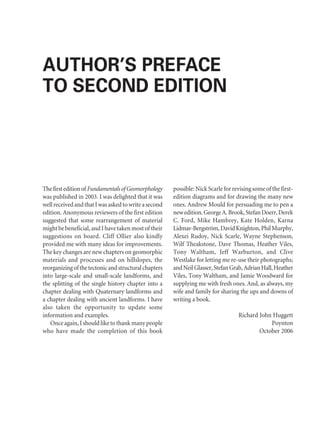
![442 PROCESS AND FORM
The study of Tertiary landscape evolution in southern Britain nicely shows how emphasis in
historical geomorphology has changed from land-surface morphology being the key to
interpretation to a more careful examination of evidence for past geomorphic processes. As Jones
(1981, 4–5) put it,
[this] radical transformation has in large part resulted from a major shift in methodology, the
heavily morphologically-biased approach of the first half of the twentieth century having
given way to studies that have concentrated on the detailed examination of superficial deposits,
including their faunal and floral content, and thereby provided a sounder basis for the dating
of geomorphological events.
The key to Wooldridge and Linton’s (1939, 1955) classic model of landscape evolution in Tertiary
south-east England was three basic surfaces, each strongly developed on the Chalkland flanks
of the London Basin (Figure 15.7). First is an inclined, recently exhumed, marine-trimmed surface
that fringes the present outcrop of Palaeogene sediments. Wooldridge and Linton called this the
Sub-Eocene Surface (it is now more accurately termed the Sub-Palaeogene surface). Second is
an undulating Summit Surface lying above about 210 m, mantled with thick residual deposits of
‘Clay-with-Flints’, and interpreted by Wooldridge and Linton as the remnants of a region-wide
subaerial peneplain, as originally suggested by Davis in 1895, rather than a high-level marine
plain lying not far above the present summits. Third is a prominent, gently inclined erosional
platform, lying between about 150 and 200 m and cutting into the Summit Surface and seemingly
truncating the Sub-Eocene Surface. As it bears sedimentary evidence of marine activity,
Wooldridge and Linton interpreted it as a Pliocene marine plain. Wooldridge and Linton believed
that the two higher surfaces – the Summit Surface and the marine platform – were not warped.
They argued, therefore, that these surfaces must have formed after the tectonic episode that
deformed the Sub-Eocene Surface, and that the summit plain had to be a peneplain fashioned
during the Miocene and Pliocene epochs.
The Wooldridge and Linton model of Tertiary landscape evolution was the ruling theory until
at least the early 1960s and perhaps as late as the early 1970s. Following Wooldridge’s death in
1963, interest in the long-term landform evolution of Britain – or denudation chronology, as many
geomorphologists facetiously dubbed it – waned. Critics accused denudation chronologists of
letting their eyes deceive them: most purely morphological evidence is ‘so ambiguous that
theory feeds readily on preconception’ (Chorley 1965, 151). However, alongside the denigration
of and declining interest in denudation chronology, some geomorphologists reappraised the
evidence for long-term landscape changes. This fresh work led in the early 1980s to the destruction
of Wooldridge and Linton’s ‘grand design’ and to the creation of a new framework that discarded
the obsession with morphological evidence in favour of the careful examination of Quaternary
deposits (Jones 1999, 5–6). The reappraisal was in part inspired by Philippe Pinchemel’s (1954)
alternative idea that the gross form of the Chalk backslopes in southern England and northern
Box 15.1 TERTIARY LANDSCAPE EVOLUTION IN SOUTH-EAST
ENGLAND
continued . . .](https://image.slidesharecdn.com/fundamentalsofgeomorphologyroutledgefundamentalsofphysicalgeography-220921044803-9a19de6c/85/fundamentalsofgeomorphology_routledgefundamentalsofphysicalgeography-pdf-461-320.jpg)


This chapter provides an introduction to the third edition of the textbook Fundamentals of Geomorphology. The author summarizes the key changes made to the book's structure based on feedback from reviewers of the second edition. These include splitting the first chapter into three sections introducing different aspects of geomorphology, rearranging material on processes and history throughout the book, and moving the chapter on karst landscapes later in the text. The author expresses his aim to integrate both process geomorphology and historical geomorphology in the book. He also thanks those who assisted with the production of the new edition.


