Introduction Frequentist Paradigm
ParametricStatistical Model
Suppose that the vector of observations x = (x1, ..., xn) is generated
from a probability distribution with density f (x | θ), where θ is the
vector of parameters.
For example, if we further assume the observations are iid, then
f (x | θ) =
n
Y
i=1
f (xi | θ) .
A parametric statistical model consists of the observation x of a
random variable X, distributed according to the density f (x | θ), where
the parameter θ belongs to a parameter space Θ of nite dimension.
Shaobo Jin (Math) Bayesian Statistics 2 / 16
3.
Introduction Frequentist Paradigm
LikelihoodFunction
Denition
For an observation x of a random variable X with density f (x | θ), the
likelihood function L (· | x) : Θ → [0, ∞) is dened by
L (θ | x) = f (x | θ).
Example
If X =
X1 · · · Xn
T
is a sample of independent random variables,
then
L (θ | x) =
n
Y
i=1
fi (xi | θ) ,
as a function in θ conditional on x.
Shaobo Jin (Math) Bayesian Statistics 3 / 16
4.
Introduction Frequentist Paradigm
LikelihoodFunction: Example
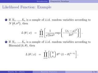
1 If X1, ..., Xn is a sample of i.i.d. random variables according to
N θ, σ2
, then
L (θ | x) =
n
Y
i=1
1
√
2πσ2
exp
(
−
(xi − µ)2
2σ2
)#
.
2 If X1, ..., Xn is a sample of i.i.d. random variables according to
Binomial (k, θ), then
L (θ | x) =
n
Y
i=1
k
xi
θxi
(1 − θ)n−xi
.
Shaobo Jin (Math) Bayesian Statistics 4 / 16
5.
Introduction Frequentist Paradigm
LikelihoodFunction: Another Example
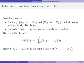
Consider the case
For i ̸= j,
Xi1 · · · Xin
and
Xj1 · · · Xjn
are independent
and identically distributed.
For each i, Xi1, ..., Xip are not necessarily independent.
Then, the likelihood is
L (θ | x) =
n
Y
i=1
f (xi1, · · · , xip | θ) ,
where f (xi1, · · · , xip | θ) is the joint density of
Xi1 · · · Xip
.
Shaobo Jin (Math) Bayesian Statistics 5 / 16
6.
Introduction Frequentist Paradigm
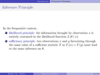
InferencePrinciple
In the frequentist context,
1 likelihood principle: the information brought by observation x is
entirely contained in the likelihood function L (θ | x).
2 suciency principle: two observations x and y factorizing through
the same value of a sucient statistic T as T (x) = T (y) must lead
to the same inference on θ.
Shaobo Jin (Math) Bayesian Statistics 6 / 16
7.
Introduction Bayesian Paradigm
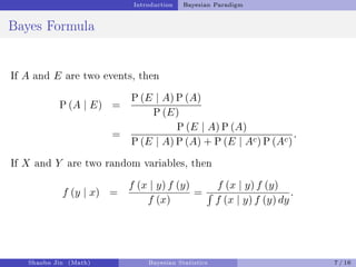
BayesFormula
If A and E are two events, then
P (A | E) =
P (E | A) P (A)
P (E)
=
P (E | A) P (A)
P (E | A) P (A) + P (E | Ac) P (Ac)
.
If X and Y are two random variables, then
f (y | x) =
f (x | y) f (y)
f (x)
=
f (x | y) f (y)
´
f (x | y) f (y) dy
.
Shaobo Jin (Math) Bayesian Statistics 7 / 16
8.
Introduction Bayesian Paradigm
Priorand Posterior
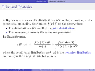
A Bayes model consists of a distribution π (θ) on the parameters, and a
conditional probability distribution f (x | θ) on the observations.
The distribution π (θ) is called the prior distribution.
The unknown parameter θ is a random parameter.
By Bayes formula,
π (θ | x) =
f (x | θ) π (θ)
m (x)
=
f (x | θ) π (θ)
´
f (x | θ) π (θ) dθ
,
where the conditional distribution π (θ | x) is the posterior distribution
and m (x) is the marginal distribution of x.
Shaobo Jin (Math) Bayesian Statistics 8 / 16
9.
Introduction Bayesian Paradigm
UpdateOur Knowledge on θ
The prior often summarizes the prior information about θ.
From similar experiences, the average number of accidents at a
crossing is 1 per 30 days. We assume
π (θ) = 30 exp (−30θ) , [day]−1
.
Our experiment resulted in an observation x.
Three accidents have been recorded after monitoring the
roundabout for one year. The likelihood is
f (X = 3 | θ) =
(365θ)3
3!
exp (−365θ) .
We use the information in x to update our knowledge on θ.
By Bayes' formula
π (θ | x) =
f (X = 3 | θ) π (θ)
m (x)
.
Shaobo Jin (Math) Bayesian Statistics 9 / 16
10.
Introduction Bayesian Paradigm
Distributions
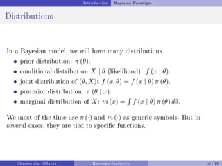
Ina Bayesian model, we will have many distributions
prior distribution: π (θ).
conditional distribution X | θ (likelihood): f (x | θ).
joint distribution of (θ, X): f (x, θ) = f (x | θ) π (θ).
posterior distribution: π (θ | x).
marginal distribution of X: m (x) =
´
f (x | θ) π (θ) dθ.
We most of the time use π (·) and m (·) as generic symbols. But in
several cases, they are tied to specic functions.
Shaobo Jin (Math) Bayesian Statistics 10 / 16
11.
Introduction Bayesian Paradigm
UseBayes Formula To Obtain Posterior
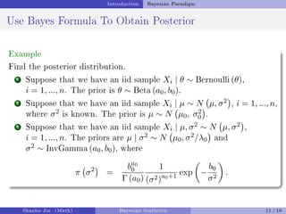
Example
Find the posterior distribution.
1 Suppose that we have an iid sample Xi | θ ∼ Bernoulli (θ),
i = 1, ..., n. The prior is θ ∼ Beta (a0, b0).
2 Suppose that we have an iid sample Xi | µ ∼ N µ, σ2
, i = 1, ..., n,
where σ2 is known. The prior is µ ∼ N µ0, σ2
0
.
3 Suppose that we have an iid sample Xi | µ, σ2 ∼ N µ, σ2
,
i = 1, ..., n. The priors are µ | σ2 ∼ N µ0, σ2/λ0
and
σ2 ∼ InvGamma (a0, b0), where
π σ2
=
ba0
0
Γ (a0)
1
(σ2)a0+1 exp
−
b0
σ2
.
Shaobo Jin (Math) Bayesian Statistics 11 / 16
12.
Introduction Bayesian Paradigm
BayesianInference Principle
Bayesian Inference Principle
Information on the underlying parameter θ is entirely contained in the
posterior distribution π (θ | x). That is, all statistical inference are
based on the posterior distribution π (θ | x).
Some examples are
1 posterior mean: E[θ | x].
2 posterior mode (MAP): θ that maximizes π (θ | x).
3 predictive distribution of a new observation:
f (y | x) =
ˆ
f (y | x, θ) π (θ | x) dθ.
Shaobo Jin (Math) Bayesian Statistics 12 / 16
13.
Introduction Multivariate NormalDistribution
From Univariate to Multivariate Normal
Let Z ∼ N (0, 1). Then, X = σZ + µ ∼ N µ, σ2
, where E [X] = µ and
Var (X) = σ2.
Let Z =
Z1 Z2 · · · Zp
T
be a random vector, each Zj ∼ N (0, 1),
and Zj is independent of Zk for any j ̸= k. Then,
X = Σ1/2
Z + µ ∈ Rp
follows a p−dimensional multivariate normal distribution, denoted by
X ∼ Np (µ, Σ), where E [X] = µ and Var (X) = Σ.
Shaobo Jin (Math) Bayesian Statistics 13 / 16
14.
Introduction Multivariate NormalDistribution
From Univariate to Multivariate Normal: Density
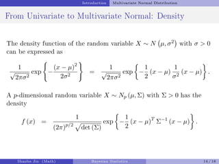
The density function of the random variable X ∼ N µ, σ2
with σ 0
can be expressed as
1
√
2πσ2
exp
(
−
(x − µ)2
2σ2
)
=
1
√
2πσ2
exp
−
1
2
(x − µ)
1
σ2
(x − µ)
.
A p-dimensional random variable X ∼ Np (µ, Σ) with Σ 0 has the
density
f (x) =
1
(2π)p/2
p
det (Σ)
exp
−
1
2
(x − µ)T
Σ−1
(x − µ)
.
Shaobo Jin (Math) Bayesian Statistics 14 / 16
15.
Introduction Multivariate NormalDistribution
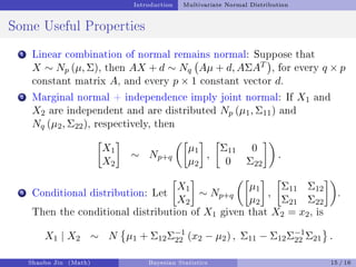
Some Useful Properties
1 Linear combination of normal remains normal: Suppose that
X ∼ Np (µ, Σ), then AX + d ∼ Nq Aµ + d, AΣAT
, for every q × p
constant matrix A, and every p × 1 constant vector d.
2 Marginal normal + independence imply joint normal: If X1 and
X2 are independent and are distributed Np (µ1, Σ11) and
Nq (µ2, Σ22), respectively, then
X1
X2
∼ Np+q
µ1
µ2
,
Σ11 0
0 Σ22
.
3 Conditional distribution: Let
X1
X2
∼ Np+q
µ1
µ2
,
Σ11 Σ12
Σ21 Σ22
.
Then the conditional distribution of X1 given that X2 = x2, is
X1 | X2 ∼ N
µ1 + Σ12Σ−1
22 (x2 − µ2) , Σ11 − Σ12Σ−1
22 Σ21 .
Shaobo Jin (Math) Bayesian Statistics 15 / 16
16.
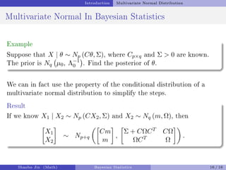
Introduction Multivariate NormalDistribution
Multivariate Normal In Bayesian Statistics
Example
Suppose that X | θ ∼ Np (Cθ, Σ), where Cp×q and Σ 0 are known.
The prior is Nq µ0, Λ−1
0
. Find the posterior of θ.
We can in fact use the property of the conditional distribution of a
multivariate normal distribution to simplify the steps.
Result
If we know X1 | X2 ∼ Np (CX2, Σ) and X2 ∼ Nq (m, Ω), then
X1
X2
∼ Np+q
Cm
m
,
Σ + CΩCT CΩ
ΩCT Ω
.
Shaobo Jin (Math) Bayesian Statistics 16 / 16
![Introduction Bayesian Paradigm
Update Our Knowledge on θ
The prior often summarizes the prior information about θ.
From similar experiences, the average number of accidents at a
crossing is 1 per 30 days. We assume
π (θ) = 30 exp (−30θ) , [day]−1
.
Our experiment resulted in an observation x.
Three accidents have been recorded after monitoring the
roundabout for one year. The likelihood is
f (X = 3 | θ) =
(365θ)3
3!
exp (−365θ) .
We use the information in x to update our knowledge on θ.
By Bayes' formula
π (θ | x) =
f (X = 3 | θ) π (θ)
m (x)
.
Shaobo Jin (Math) Bayesian Statistics 9 / 16](https://image.slidesharecdn.com/lecture1introduction-250729102714-2429e69f/85/bayesian_statistics_introduction_uppsala_university-9-320.jpg)
![Introduction Bayesian Paradigm
Bayesian Inference Principle
Bayesian Inference Principle
Information on the underlying parameter θ is entirely contained in the
posterior distribution π (θ | x). That is, all statistical inference are
based on the posterior distribution π (θ | x).
Some examples are
1 posterior mean: E[θ | x].
2 posterior mode (MAP): θ that maximizes π (θ | x).
3 predictive distribution of a new observation:
f (y | x) =
ˆ
f (y | x, θ) π (θ | x) dθ.
Shaobo Jin (Math) Bayesian Statistics 12 / 16](https://image.slidesharecdn.com/lecture1introduction-250729102714-2429e69f/85/bayesian_statistics_introduction_uppsala_university-12-320.jpg)
![Introduction Multivariate Normal Distribution
From Univariate to Multivariate Normal
Let Z ∼ N (0, 1). Then, X = σZ + µ ∼ N µ, σ2
, where E [X] = µ and
Var (X) = σ2.
Let Z =
Z1 Z2 · · · Zp
T
be a random vector, each Zj ∼ N (0, 1),
and Zj is independent of Zk for any j ̸= k. Then,
X = Σ1/2
Z + µ ∈ Rp
follows a p−dimensional multivariate normal distribution, denoted by
X ∼ Np (µ, Σ), where E [X] = µ and Var (X) = Σ.
Shaobo Jin (Math) Bayesian Statistics 13 / 16](https://image.slidesharecdn.com/lecture1introduction-250729102714-2429e69f/85/bayesian_statistics_introduction_uppsala_university-13-320.jpg)


![ANIMAL_CELL_,_TISSUE_AND_ORGAN_CULTURE[1].pptx](https://cdn.slidesharecdn.com/ss_thumbnails/animalcelltissueandorganculture1-260204172026-4462b440-thumbnail.jpg?width=640&height=640&fit=bounds)


