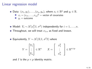
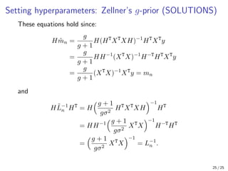
The document provides an in-depth overview of Bayesian linear regression, discussing the model, prior and posterior distributions, and various settings of hyperparameters including unit information and Zellner’s g-prior. It highlights the connections between Bayesian methods and frequentist approaches like maximum likelihood estimation and ridge regression, as well as the use of conjugate priors for efficient inference. Moreover, it introduces the Gibbs sampler for joint inference and outlines the advantages of Monte Carlo methods over MCMC for posterior computation.

1. Bayesian linear regression
Bayesian Methodology in Biostatistics (BST 249)
Jeffrey W. Miller
Department of Biostatistics
Harvard T.H. Chan School of Public Health
1 / 25

2. Outline
Model, prior, and posterior
Conditionally conjugate prior on β
Conditionally conjugate prior on σ2
Setting the hyperparameters
Unit information prior
Zellner’s g-prior
Computation with Zellner’s g-prior
2 / 25

3. Outline
Model, prior, and posterior
Conditionally conjugate prior on β
Conditionally conjugate prior on σ2
Setting the hyperparameters
Unit information prior
Zellner’s g-prior
Computation with Zellner’s g-prior
3 / 25

4. Linear regression model
Data: (x1, y1), . . . , (xn, yn), where xi ∈ Rp and yi ∈ R.
I xi = (xi1, . . . , xip)T
= vector of covariates
I yi = outcome
Model: Yi ∼ N(xT
i β, σ2) independently for i = 1, . . . , n.
Throughout, we will treat x1:n as fixed and known.
Equivalently, Y ∼ N(Xβ, σ2I) where
Y =



Y1
.
.
.
Yn


 ∈ Rn
X =



xT
1
.
.
.
xT
n


 ∈ Rn×p
and I is the p × p identity matrix.
4 / 25

5. Conditionally conjugate prior on β
Assume a multivariate normal prior on β:
β ∼ N(m0, L−1
0 ).
For any fixed σ2, this is a conjugate prior.
The resulting posterior, with σ2 fixed, is:
β|y1:n ∼ N(mn, L−1
n )
where
Ln = L0 + XT
X/σ2
,
mn = L−1
n (L0m0 + XT
y/σ2
),
and y = (y1, . . . , yn)T ∈ Rn.
5 / 25

6. Connections with the MLE and ridge regression
The maximum a posteriori (MAP) estimate is the mode of
the posterior.
Since the posterior is normal, the mode is equal to the mean:
β̂MAP = mn = (L0 + XT
X/σ2
)−1
(L0m0 + XT
y/σ2
).
In the limit as L0 → 0, we have Ln → XTX/σ2 and
β̂MAP = mn → (XT
X)−1
XT
y = β̂MLE.
Thus, in the limit of having “no prior information” about β,
β|y1:n ∼ N(β̂MLE, σ2
(XT
X)−1
).
Note that the frequentist sampling distribution of the MLE is
β̂MLE ∼ N(β, σ2
(XT
X)−1
)
when β is the true parameter, which exhibits perfect
symmetry with the posterior above when we take L0 → 0.
6 / 25

7. Connections with the MLE and ridge regression
Taking L0 → 0 is equivalent to using a flat prior p(β) ∝ 1
and formally applying Bayes’ theorem: p(β|y1:n) ∝ p(y1:n|β).
p(β) ∝ 1 is called an improper prior since it cannot be
normalized to a probability density on Rp.
Even though the flat prior on β is improper, defining
p(β|y1:n) ∝ p(y1:n|β) still results in a well-defined posterior
distribution as long as n ≥ 1.
This is an example of a noninformative prior.
The MAP estimate also generalizes ridge regression.
Specifically, if m0 = 0 and L0 = αI/σ2 then
β̂MAP = (XT
X + αI)−1
XT
y = β̂ridge.
7 / 25

8. Outline
Model, prior, and posterior
Conditionally conjugate prior on β
Conditionally conjugate prior on σ2
Setting the hyperparameters
Unit information prior
Zellner’s g-prior
Computation with Zellner’s g-prior
8 / 25

9. Conjugate prior on σ2
Similar to the case of a univariate normal model, the Inverse
Gamma distribution is a conjugate prior for σ2.
Suppose β is fixed, and define the prior on σ2 as:
σ2
∼ InvGamma 1
2ν0, 1
2ν0σ2
0
.
This parametrization facilitates interpretation:
I σ2
0 = prior guess of σ2
(since σ0 is between the mean and the
mode of this prior on σ2
)
I ν0 = confidence in the choice of σ2
0, in units of sample size —
i.e., the strength of the prior is equivalent to ν0 samples.
The resulting posterior on σ2 is then
σ2
|y1:n ∼ ???
(Whiteboard activity)
9 / 25

10. Conjugate prior on σ2
Similar to the case of a univariate normal model, the Inverse
Gamma distribution is a conjugate prior for σ2.
Suppose β is fixed, and define the prior on σ2 as:
σ2
∼ InvGamma 1
2ν0, 1
2ν0σ2
0
.
This parametrization facilitates interpretation:
I σ2
0 = prior guess of σ2
(since σ0 is between the mean and the
mode of this prior on σ2
)
I ν0 = confidence in the choice of σ2
0, in units of sample size —
i.e., the strength of the prior is equivalent to ν0 samples.
The resulting posterior on σ2 is then
σ2
|y1:n ∼ InvGamma 1
2(ν0 + n), 1
2(ν0σ2
0 + SSR(β)
where SSR(β) =
Pn
i=1(yi − xT
i β)2.
10 / 25

11. Inference for β and σ2
jointly
We’ve seen conjugate priors for β and σ2, given the other.
Thus, these define a conditionally conjugate prior, combined:
β ∼ N(m0, L−1
0 ) σ2
∼ InvGamma 1
2ν0, 1
2ν0σ2
0
independently.
We know how to compute β|σ2, y1:n and σ2|β, y1:n. How can
we infer β and σ2 jointly?
One way: Initialize β, σ2 and iteratively repeat the following:
1. update β by sampling from β|σ2
, y1:n
2. update σ2
by sampling from σ2
|β, y1:n
It turns out that this generates approximate samples from
β, σ2|y1:n. This is an example of a Gibbs sampler, which is
type of a Markov chain Monte Carlo algorithm.
11 / 25

12. Group activity: Statistics trivia challenge!
Go to breakout rooms and work together to answer these questions:
https://forms.gle/agm9P7PpLTWNUmDr5
(Three people per room, randomly assigned. 5 minutes.)
12 / 25

13. Outline
Model, prior, and posterior
Conditionally conjugate prior on β
Conditionally conjugate prior on σ2
Setting the hyperparameters
Unit information prior
Zellner’s g-prior
Computation with Zellner’s g-prior
13 / 25

14. Setting hyperparameters: Data-dependent, Unit info
The subjective Bayesian approach is to set hyperparameters
based solely on prior beliefs. However, sometimes we prefer to
use default priors that don’t require subjective input.
Data-dependent priors are a useful way of creating default
priors, even though, strictly speaking, they violate the
principle of not using the data twice.
Kass Wasserman (1995) propose the following settings:
m0 = β̂MLE L0 = XT
X/(nσ2
).
Similarly, we can define a data-dependent prior on σ2:
σ2
0 = σ̂2
MLE ν0 = 1
where σ̂2
MLE is the maximum likelihood estimate of σ2.
These are both unit information priors — the strength of the
prior is equivalent to one sample.
14 / 25

15. Setting hyperparameters: Zellner’s g-prior
A compelling property of β̂MLE is that the scale of the
predictors doesn’t matter, in the following sense:
I Suppose one of the predictors is age in years.
I If we change the units of age to months, then entry of β̂MLE
corresponding to age is scaled accordingly by 1/12.
I Consequently, Xβ̂MLE is invariant to the choice of units.
Mathematically, changing the units means using the model
Y ∼ N(X̃β, σ2I) with X̃ = XH in place of X, where H is a
diagonal matrix with Hjj 0 for all j. Observe that
X̃
˜
β̂MLE = ??? = Xβ̂MLE.
(Whiteboard activity)
15 / 25

16. Setting hyperparameters: Zellner’s g-prior
A compelling property of β̂MLE is that the scale of the
predictors doesn’t matter, in the following sense:
I Suppose one of the predictors is age in years.
I If we change the units of age to months, then entry of β̂MLE
corresponding to age is scaled accordingly by 1/12.
I Consequently, Xβ̂MLE is invariant to the choice of units.
Mathematically, changing the units means using the model
Y ∼ N(X̃β, σ2I) with X̃ = XH in place of X, where H is a
diagonal matrix with Hjj 0 for all j. Observe that
X̃
˜
β̂MLE = X̃(X̃T
X̃)−1
X̃T
y
= XH(HT
XT
XH)−1
HT
XT
y
= XHH−1
(XT
X)−1
H−T
HT
XT
y
= X(XT
X)−1
XT
y = Xβ̂MLE.
16 / 25

17. Setting hyperparameters: Zellner’s g-prior
This is nice since, intuitively, the units shouldn’t matter.
For the Bayesian model, the invariance property we seek is:
I Suppose X̃ = XH for some invertible H ∈ Rp×p
.
I Let β be distributed according to the posterior using X.
I Let β̃ be distributed according to the posterior using X̃.
I We would like Xβ and X̃β̃ to have the same distribution.
Unfortunately, for most choices of prior, the posterior doesn’t
have this invariance property.
However, if we can make it so that β and Hβ̃ have the same
distribution, then this will work, since then Xβ has the same
distribution as XHβ̃ = X̃β̃.
17 / 25

18. Setting hyperparameters: Zellner’s g-prior
This invariance property is satisfied by Zellner’s g-prior:
β|σ2
∼ N(m0, L−1
0 ) where m0 = 0 and L0 = XT
X/(gσ2
).
Here, g 0 is a free parameter.
Given σ2, the posterior on β under a g-prior simplifies to:
β | σ2
, y1:n ∼ N(mn, L−1
n )
where
Ln = L0 + XT
X/σ2
=
g + 1
gσ2
XT
X,
mn = L−1
n (L0m0 + XT
y/σ2
) =
g
g + 1
(XT
X)−1
XT
y.
18 / 25

19. Setting hyperparameters: Zellner’s g-prior
To check that the invariance property is satisfied, suppose:
m̃0 = 0 L̃0 = (XH)T
(XH)/(gσ2
).
Then the posterior is β̃ | σ2, y1:n ∼ N(m̃n, L̃−1
n ) where
L̃n = ???
m̃n = ???.
Since Hβ̃ | σ2, y1:n ∼ N(???, ???), the invariance property
requires that
Hm̃n = mn and HL̃−1
n HT
= L−1
n .
Group activity: Go to breakout rooms and work together
to (1) fill in the blanks above and (2) check that the
equations above in red hold. (15 minutes)
19 / 25

20. Outline
Model, prior, and posterior
Conditionally conjugate prior on β
Conditionally conjugate prior on σ2
Setting the hyperparameters
Unit information prior
Zellner’s g-prior
Computation with Zellner’s g-prior
20 / 25

21. Posterior computation with Zellner’s g-prior
The g-prior also simplifies posterior inference for (β, σ2).
Assume a g-prior on β|σ2 and an InvGamma prior on σ2:
β|σ2
∼ N 0, gσ2
(XT
X)−1
σ2
∼ InvGamma 1
2ν0, 1
2ν0σ2
0
.
It turns out that we can generate i.i.d. samples from the
posterior on (β, σ2), so we don’t need to use MCMC.
These samples can be used for Monte Carlo approximation of
posterior expectations, e.g., for any integrable function h,
E(h(β, σ2
) | y1:n) ≈
1
T
T
X
t=1
h(βt, σ2
t ).
Monte Carlo has various advantages over MCMC: simplicity,
efficiency, and reliable quantification of approximation error.
21 / 25

22. Posterior computation with Zellner’s g-prior
Under the prior on the previous slide, it can be shown that the
posterior is (Hoff, 2009):
σ2
| y1:n ∼ InvGamma
1
2(ν0 + n), 1
2(ν0σ2
0 + SSRg)
β | σ2
, y1:n ∼ N
g
g + 1
β̂MLE,
g
g + 1
σ2
(XT
X)−1
where
SSRg = yT
y −
g
g + 1
yT
X(XT
X)−1
XT
y.
Thus, we can generate i.i.d. samples from the posterior by:
1. sampling σ2
| y1:n,
2. sampling β | σ2
, y1:n.
22 / 25

23. References and supplements
Hoff, P. D. (2009). A First Course in Bayesian Statistical
Methods. Springer, New York.
Kass, R. E., Wasserman, L. (1995). A reference Bayesian
test for nested hypotheses and its relationship to the Schwarz
criterion. Journal of the American Statistical Association,
90(431), 928-934.
Zellner, A. (1986). On assessing prior distributions and
Bayesian regression analysis with g-prior distributions. In:
Bayesian inference and Decision Techniques, vol 6,
North-Holland, Amsterdam, 233-243.
23 / 25

24. Setting hyperparameters: Zellner’s g-prior (SOLUTIONS)
To check that the invariance property is satisfied, suppose:
m̃0 = 0 L̃0 = (XH)T
(XH)/(gσ2
).
Then the posterior is β̃ | σ2, y1:n ∼ N(m̃n, L̃−1
n ) where
L̃n =
g + 1
gσ2
HT
XT
XH
m̃n =
g
g + 1
(HT
XT
XH)−1
HT
XT
y.
Since Hβ̃ | σ2, y1:n ∼ N(Hm̃n, HL̃−1HT), the invariance
property requires that
Hm̃n = mn and HL̃−1
n HT
= L−1
n .
24 / 25

25. Setting hyperparameters: Zellner’s g-prior (SOLUTIONS)
These equations hold since:
Hm̃n =
g
g + 1
H(HT
XT
XH)−1
HT
XT
y
=
g
g + 1
HH−1
(XT
X)−1
H−T
HT
XT
y
=
g
g + 1
(XT
X)−1
XT
y = mn
and
HL̃−1
n HT
= H
g + 1
gσ2
HT
XT
XH
−1
HT
= HH−1
g + 1
gσ2
XT
X
−1
H−T
HT
=
g + 1
gσ2
XT
X
−1
= L−1
n .
25 / 25