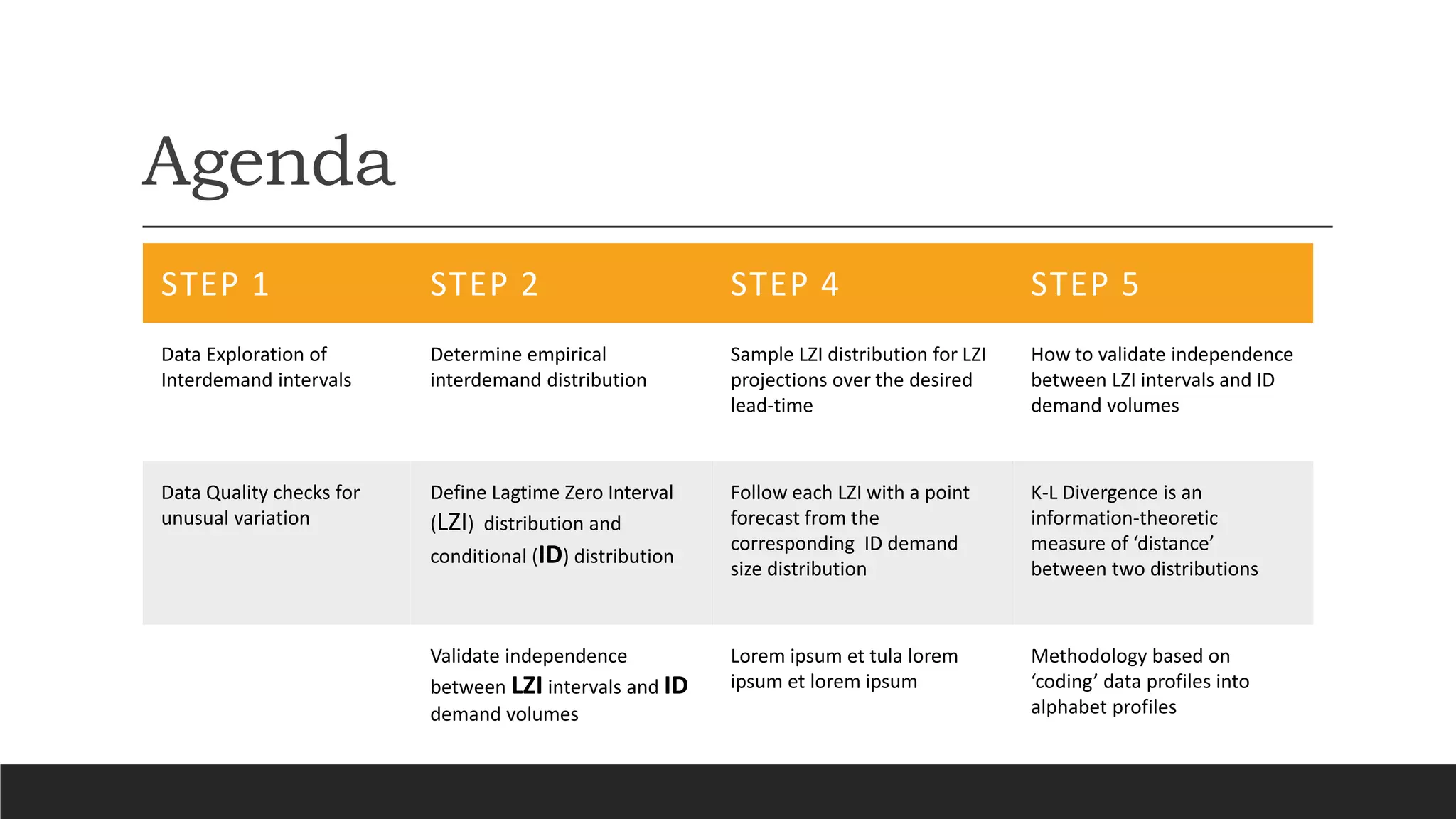
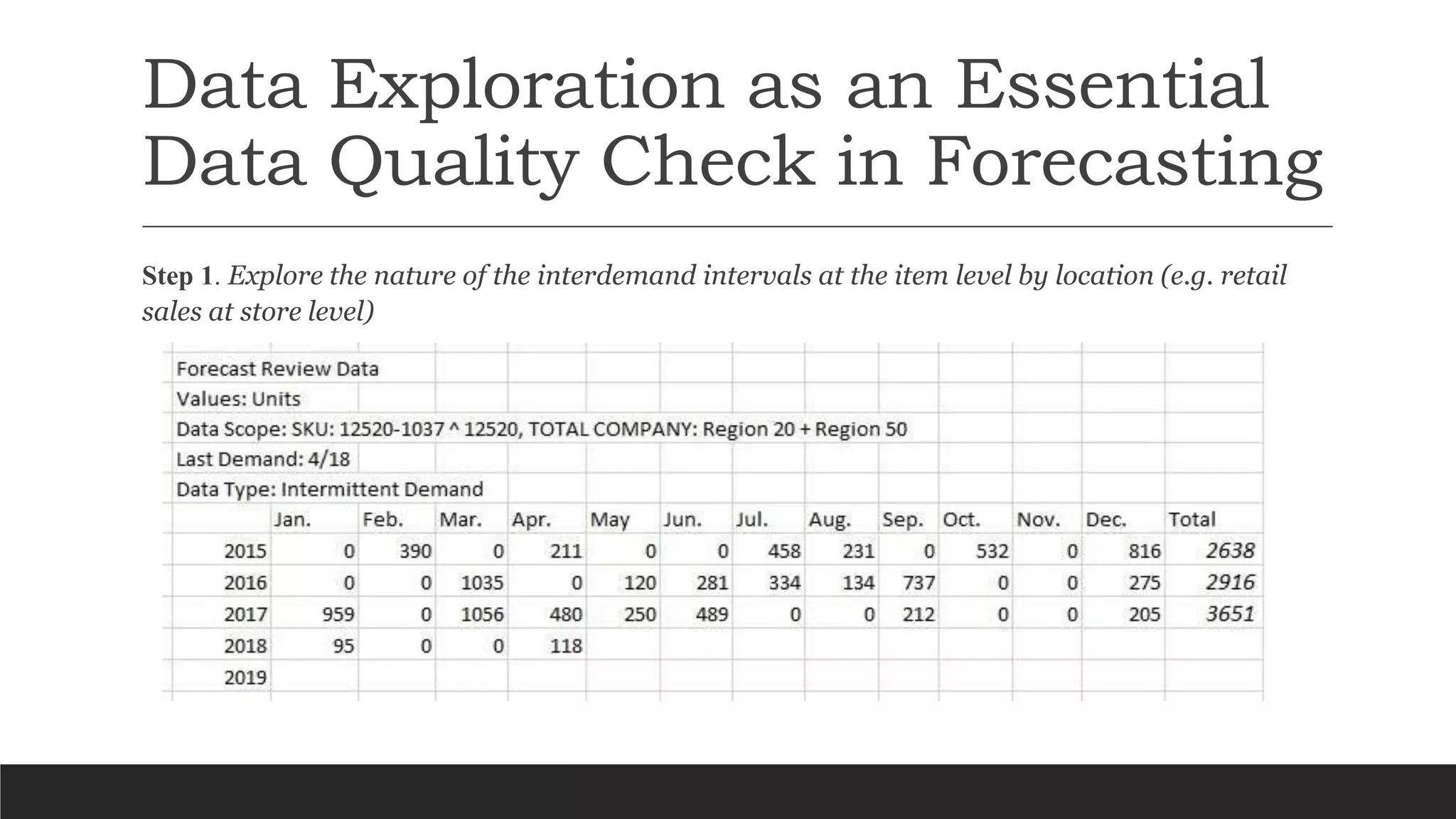
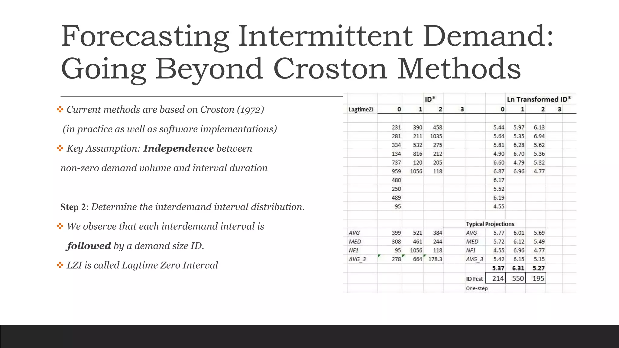
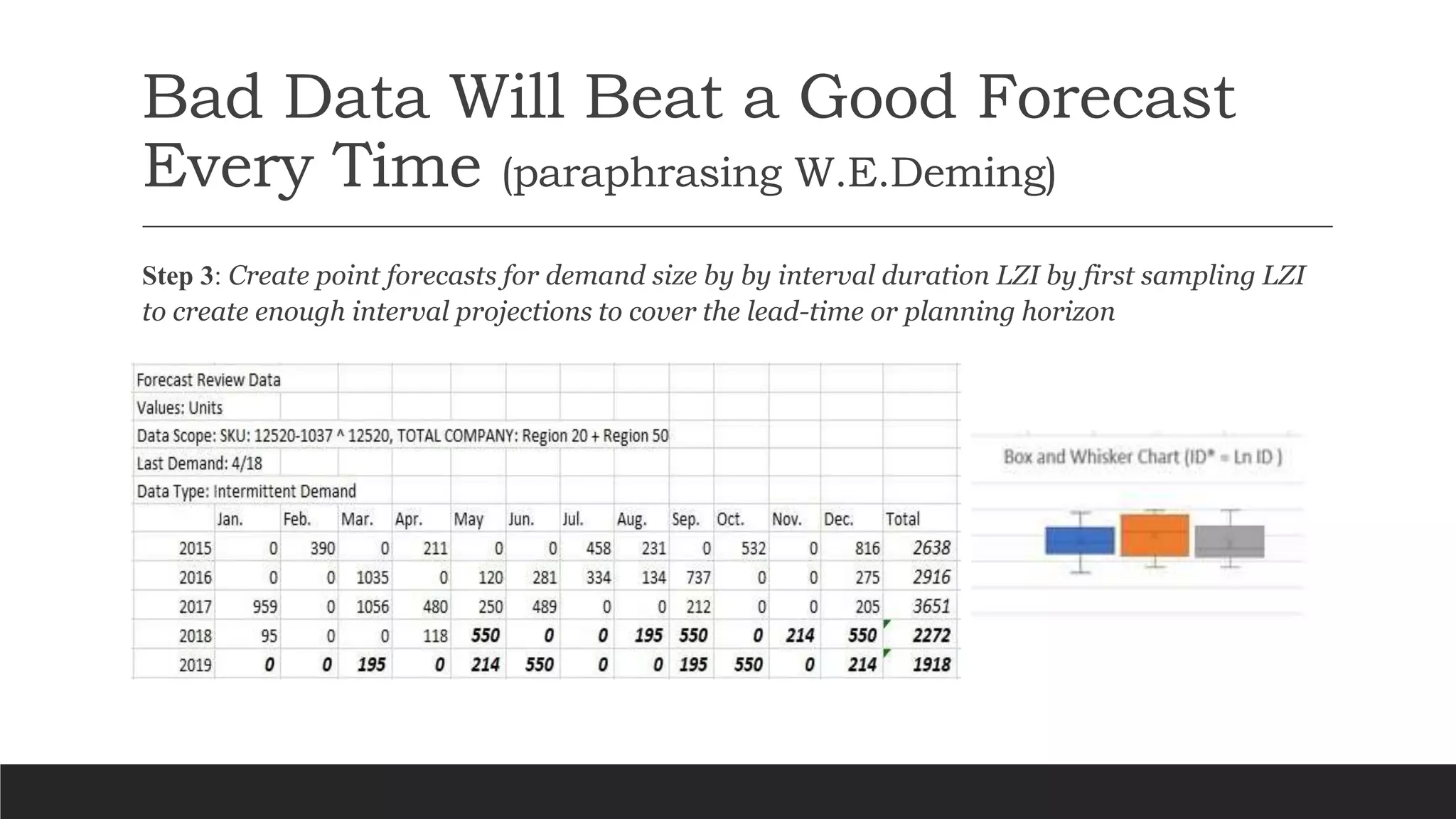
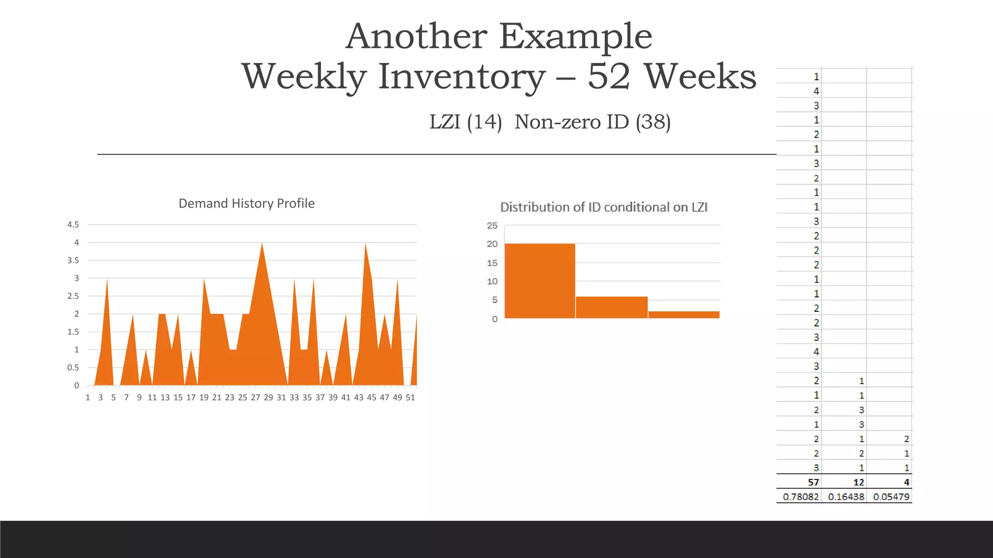
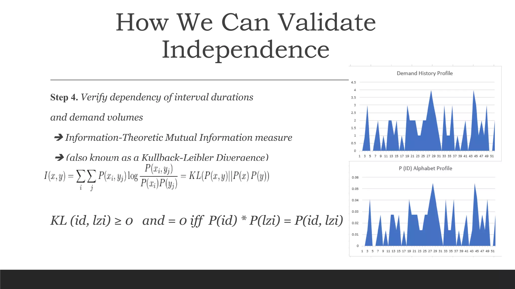
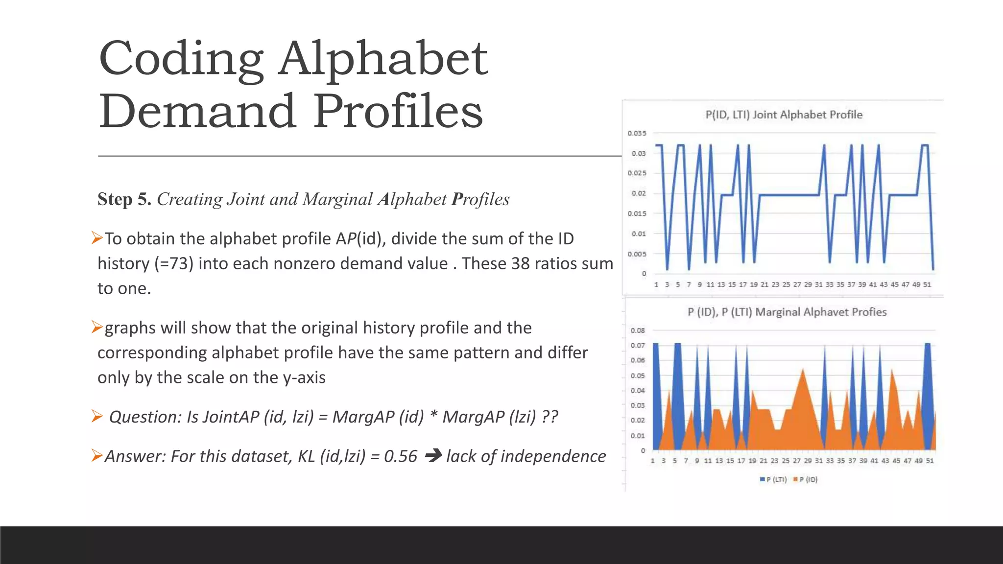
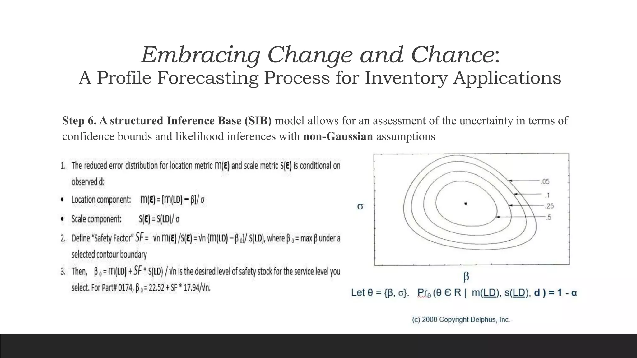
The document discusses a new approach to forecasting intermittent demand, criticizing previous reliance on traditional methods like Croston's due to their assumption of independence between demand sizes and intervals. It proposes a data-driven, non-Gaussian modeling approach utilizing empirical distributions and mutual information measures to validate independence. Key steps include exploring interdemand intervals, sampling distributions, and creating joint and marginal alphabet profiles to improve forecast accuracy.

1. Forecasting
with
Intermittent
Demand –
A New Approach
HANS LEVENBACH
ISIS SANTOS COSTA

2. In IJF, Almost Three Decades Ago Now
. . .
The signal failure on the part of statisticians to respond to the model building failures identified in many
empirical studies (..on forecast accuracy measurement..) has not been resolved within the forecasting
profession itself. Robert Fildes, IJF 8 (1992), 1-2.
The focus in forecast evaluation should be shifted from a measure-oriented approach to a distributions-
oriented approach in which distributions are primary and other measures are viewed as summarizing
different aspects of the distributions. Allan H. Murphy and Robert Winkler, IJF 8 (1992), 105-07,
A particularly sobering finding is the poor performance of the RMSE. The reliability of the RMSE is poor
(in forecasting) and it is scale dependent. Dennis A. Ahlburg, IJF 8 (1992). 99-100.

3. Agenda
STEP 1 STEP 2 STEP 4 STEP 5
Data Exploration of
Interdemand intervals
Determine empirical
interdemand distribution
Sample LZI distribution for LZI
projections over the desired
lead-time
How to validate independence
between LZI intervals and ID
demand volumes
Data Quality checks for
unusual variation
Define Lagtime Zero Interval
(LZI) distribution and
conditional (ID) distribution
Follow each LZI with a point
forecast from the
corresponding ID demand
size distribution
K-L Divergence is an
information-theoretic
measure of ‘distance’
between two distributions
Validate independence
between LZI intervals and ID
demand volumes
Lorem ipsum et tula lorem
ipsum et lorem ipsum
Methodology based on
‘coding’ data profiles into
alphabet profiles

4. Data Exploration as an Essential
Data Quality Check in Forecasting
Step 1. Explore the nature of the interdemand intervals at the item level by location (e.g. retail
sales at store level)

5. Forecasting Intermittent Demand:
Going Beyond Croston Methods
 Current methods are based on Croston (1972)
(in practice as well as software implementations)
 Key Assumption: Independence between
non-zero demand volume and interval duration
Step 2: Determine the interdemand interval distribution.
 We observe that each interdemand interval is
followed by a demand size ID.
 LZI is called Lagtime Zero Interval

6. Bad Data Will Beat a Good Forecast
Every Time (paraphrasing W.E.Deming)
Step 3: Create point forecasts for demand size by by interval duration LZI by first sampling LZI
to create enough interval projections to cover the lead-time or planning horizon

7. Another Example
Weekly Inventory – 52 Weeks
LZI (14) Non-zero ID (38)
0
0.5
1
1.5
2
2.5
3
3.5
4
4.5
1 3 5 7 9 11 13 15 17 19 21 23 25 27 29 31 33 35 37 39 41 43 45 47 49 51
Demand History Profile

8. How We Can Validate
Independence
Step 4. Verify dependency of interval durations
and demand volumes
 Information-Theoretic Mutual Information measure
 (also known as a Kullback-Leibler Divergence)
KL (id, lzi) ≥ 0 and = 0 iff P(id) * P(lzi) = P(id, lzi)

9. Coding Alphabet
Demand Profiles
Step 5. Creating Joint and Marginal Alphabet Profiles
To obtain the alphabet profile AP(id), divide the sum of the ID
history (=73) into each nonzero demand value . These 38 ratios sum
to one.
graphs will show that the original history profile and the
corresponding alphabet profile have the same pattern and differ
only by the scale on the y-axis
 Question: Is JointAP (id, lzi) = MargAP (id) * MargAP (lzi) ??
Answer: For this dataset, KL (id,lzi) = 0.56  lack of independence

10. Embracing Change and Chance:
A Profile Forecasting Process for Inventory Applications
Step 6. A structured Inference Base (SIB) model allows for an assessment of the uncertainty in terms of
confidence bounds and likelihood inferences with non-Gaussian assumptions

11. Final Takeaway
A data-driven non-Gaussian modeling approach for lead-time intermittent demand
forecasting is based on
 No independence assumptions made on demand size and demand interval distributions as
required with Croston methods.
Using bootstrap resampling (MCMC) of the underlying empirical distributions are used to
generate lagtime zero intervals (LZI). Each interval is followed by a non-zero demand (ID)
from a conditional distribution
 Independence or lack thereof can be measured with a Mutual Information (Kullback-
Leibler Divergence) measure

12. Approach Added to On Demand Paperback Book &
Professional Development Workshop Manual
Available online from Amazon.com
Paperback book
https://amzn.to/2HTAU3l
Workshop Manual
https://amzn.to/2tAhoE0