The document discusses flexible alternating current transmission systems (FACTS) with a focus on static shunt compensation and its objectives like voltage regulation, stability improvement, and power oscillation damping. It explains methods of controllable VAR generation and details the importance of midpoint shunt compensation for enhancing transmission capacity and voltage stability. Additionally, it outlines the characteristics and requirements of compensators to maintain synchronous operation and improve system performance under various load conditions.

1. Flexible Alternating Current Transmission System
(FACTS)
Presented by
G.MADHURI,
Assistant Professor(C),
Department of EEE, JNTUHCEM.
madhurigundenm@gmail.com

2. Static Shunt Compensation:
Objectives of shunt compensation.
Midpoint voltage regulation.
Voltage instability prevention.
Improvement of transient stability.
Power oscillation damping.
Methods of controllable var generation
Variable impedance type static var generators.
switching converter type var generators.
Hybrid var generators.

3.  Reactive compensation makes transmission line more compatible with load demand.
• The main objective of shunt compensation is
To increase power transmitted
Increase system stability
Reduce losses
Voltage regulation
Dynamic voltage control
Damp power oscillations
 If the power system is lightly loaded  fixed or mechanically switched shunt reactors
is used to maintain voltage level. If the power system is heavily loaded  fixed or
mechanically switched shunt capacitors is used.
OBJECTIVES OF SHUNT COMPENSATION

4. • Var compensation is used for voltage regulation at the midpoint (or some
intermediate) to segment the transmission line.
• At the end of the (radial) line to prevent voltage instability, as well as for dynamic
voltage control to increase transient stability and "damp power oscillations.
• Examples of shunt compensation is STATCOM and SVC.
OBJECTIVES OF SHUNT COMPENSATION

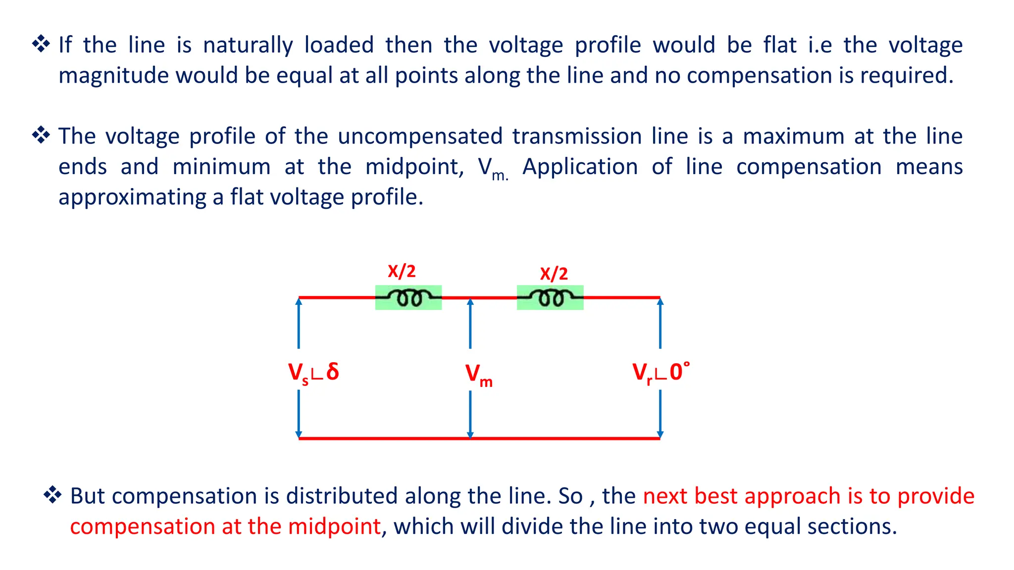
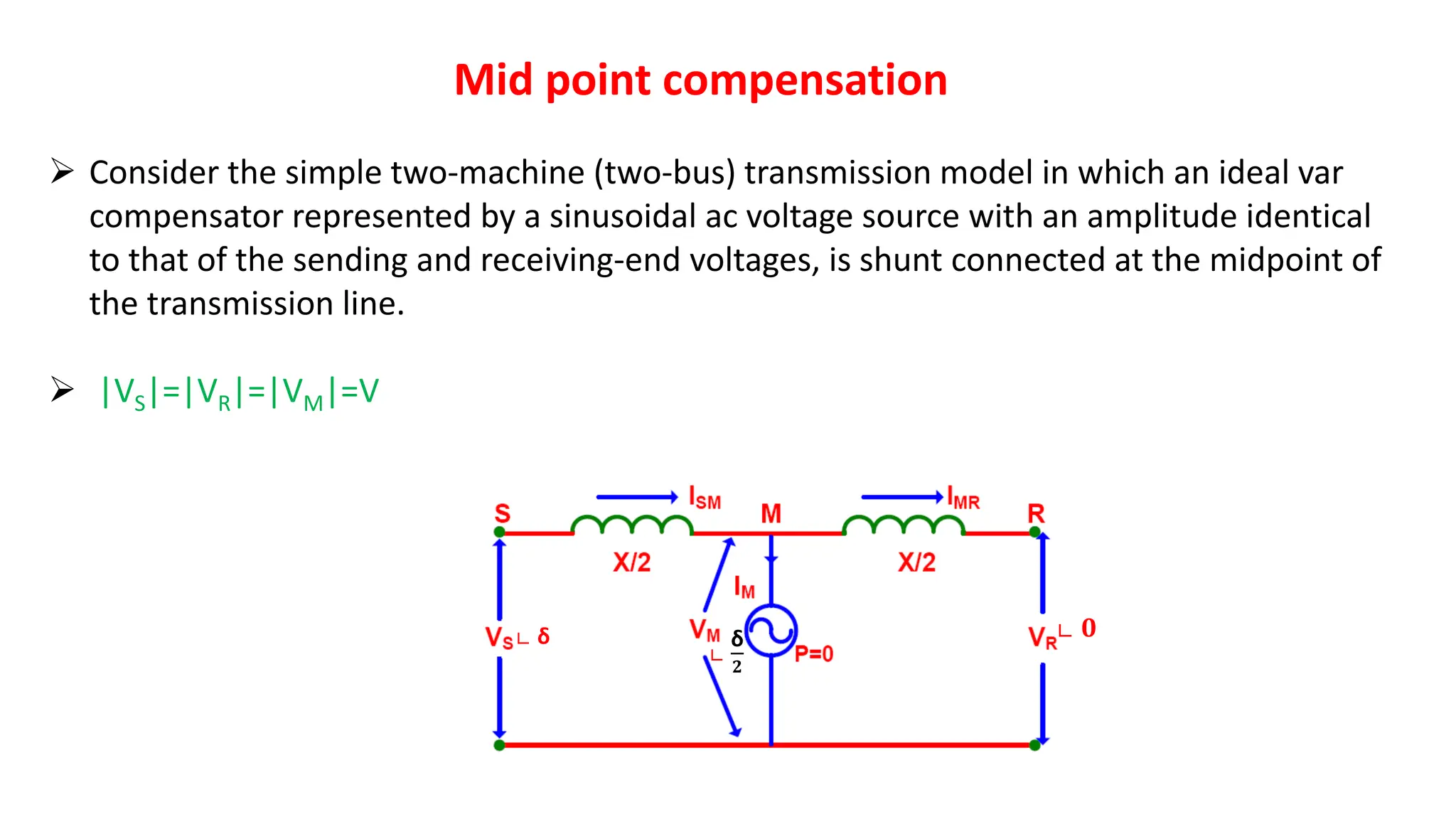
5. Midpoint Voltage Regulation for Line Segmentation
Uncompensated Case: Let us consider a simplified model of the uncompensated system.
Power = Sr=Vr Ir* =Vr [
Vs∟δ − Vr∟0˚
𝒋𝑿
]*
Vr∟0˚
Vs∟
δ
X
I
Vs∟δ
Vr∟0˚
Vx
δ
I

6. Sr=Vr Ir* = Vr [
Vs∟δ − Vr∟0˚
𝑗𝑋
]* = Vr [
Vs∟δ
𝑗𝑋
−
Vr∟0˚
𝑗𝑋
]*
= Vr [
Vs∟(δ−90)
𝑋
−
Vr∟90˚
𝑋
]* = Vr [
Vs∟(90−δ)
𝑋
−
Vr∟90˚
𝑋
]
=
VrVs∟(90−δ)
𝑋
−
Vr2∟90˚
𝑋
Pr =
VrVsCos(90−δ)
𝑋
−
Vr2Cos90˚
𝑋
=
VrVsSinδ
𝑋
------------------------------------------1
Qr =
VrVsSin(90−δ)
𝑋
−
Vr2Sin90˚
𝑋
=
VrVsCosδ)
𝑋
−
Vr2
𝑋
Qr =
Vr
𝑋
(VsCosδ − Vr) −−−−−−−−−−−−−−−−−−−−2
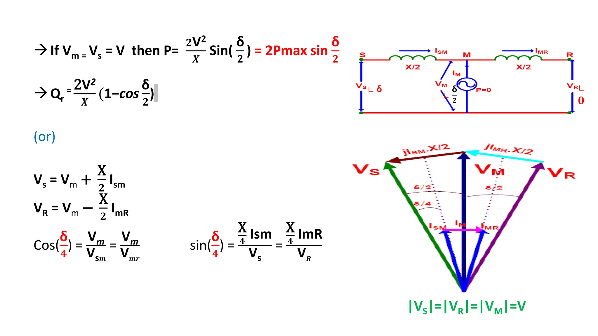
If Vr = Vs = V then P=(V2/X) Sinδ = Pmax sinδ
Qr
= V2
𝑿
(Cosδ − 1)

7.  If the line is naturally loaded then the voltage profile would be flat i.e the voltage
magnitude would be equal at all points along the line and no compensation is required.
 The voltage profile of the uncompensated transmission line is a maximum at the line
ends and minimum at the midpoint, Vm. Application of line compensation means
approximating a flat voltage profile.
Vs∟δ Vr∟0˚
Vm
X/2 X/2
 But compensation is distributed along the line. So , the next best approach is to provide
compensation at the midpoint, which will divide the line into two equal sections.

8.  Consider the simple two-machine (two-bus) transmission model in which an ideal var
compensator represented by a sinusoidal ac voltage source with an amplitude identical
to that of the sending and receiving-end voltages, is shunt connected at the midpoint of
the transmission line.
 |VS|=|VR|=|VM|=V
Mid point compensation
∟
δ
𝟐
∟ δ ∟ 𝟎

9.  The midpoint compensator in effect segments the transmission line into two
independent parts: The first segment, with an impedance of X/2, carries power from
the sending end to the midpoint, and the second segment, also with an impedance of
X/2, carries power from the midpoint to the receiving end.
 The midpoint VAR compensator exchanges only reactive power with the transmission
line in this process. The compensator does not consume any real power (P=0) since the
compensator voltage VM, and its current IM are in quadrature.
 For the lossless system assumed, the real power is the same at each terminal (sending
end, midpoint, and receiving end) of the line.

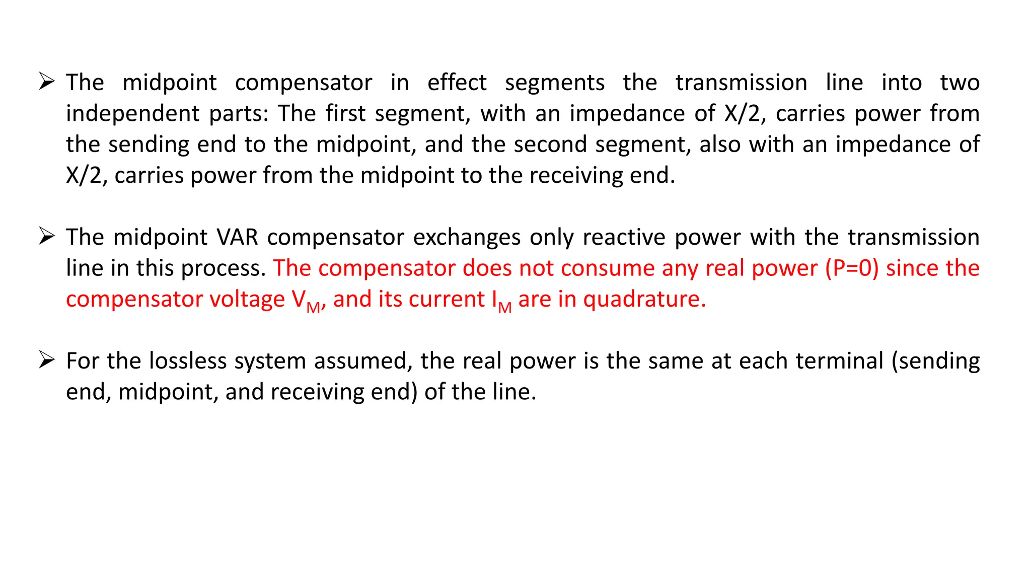
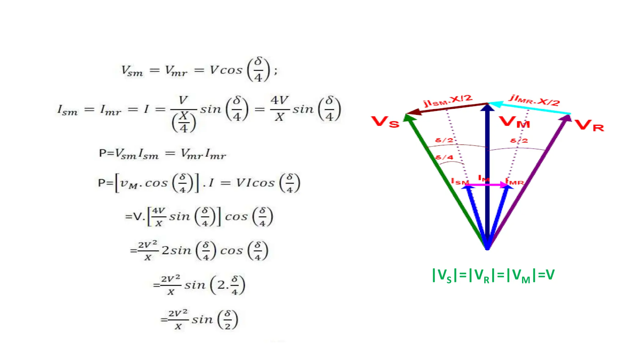
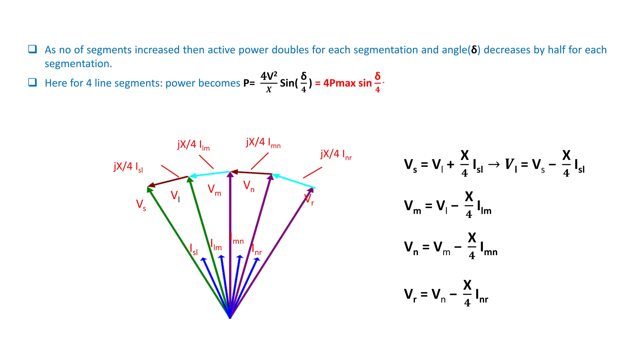
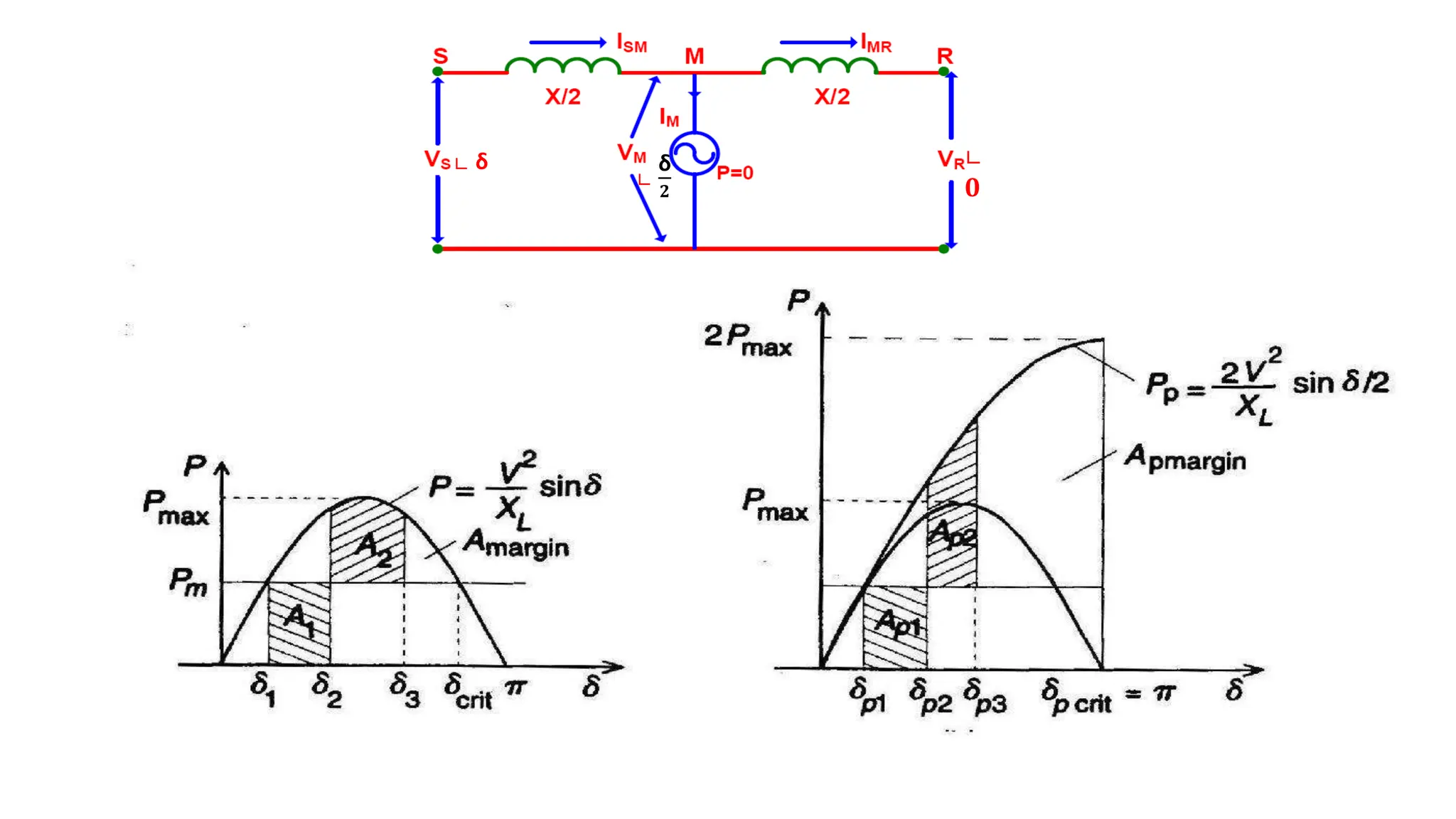
10. Sr=Vr Ir* = Vs∟δ [
Vs∟δ − Vm∟δ/𝟐˚
𝒋𝑿/𝟐
]* = Vs∟δ [
Vs∟δ
𝒋𝑿/𝟐
−
V̊m∟δ/𝟐
𝒋𝑿/𝟐
]*
= Vs∟δ [
Vs∟(δ−𝟗𝟎)
𝑿/𝟐
−
Vm∟(δ
𝟐
−𝟗𝟎)
𝑿/𝟐
]* = Vs∟δ [
Vs∟(90−δ)
𝑿/𝟐
−
Vm∟(90−δ
𝟐
)
𝑿
𝟐
]
=
Vs
2∟(90−δ+δ)
𝑿/𝟐
−
VmVs∟(90−δ
𝟐
+δ)
𝑿
𝟐
=
Vs
2∟(𝟗𝟎)
𝑿/𝟐
−
VmVs∟(90+δ
𝟐
)
𝑿
𝟐
Pr =
Vs
2cos(𝟗𝟎)
𝑿/𝟐
−
VmVscos(90+δ
𝟐
)
𝑿
𝟐
=−
VmVs(−𝐬𝐢𝐧
δ
𝟐
)
𝑿
𝟐
=
2VmVs𝒔𝒊𝒏
δ
𝟐
𝑿
Qr =
Vs
2sin(𝟗𝟎)
𝑿/𝟐
−
VmVssin(90+δ
𝟐
)
𝑿
𝟐
=
𝟐Vs
2
𝑿
−
2VmVscosδ
𝟐
𝑿
=
2Vs
𝑿
(Vs − Vmcos
δ
𝟐
).

11. ∟
δ
𝟐
∟ δ ∟
𝟎
|VS|=|VR|=|VM|=V
If Vm = Vs = V then P=
𝟐V2
𝑿
Sin(
δ
𝟐
) = 2Pmax sin
δ
𝟐
Qr
= 2V2
𝑿
(1−cos
δ
𝟐
)
(or)
Vs = Vm +
X
𝟐
Ism
VR = Vm −
X
𝟐
ImR
Cos(
δ
𝟒
) =
Vm
Vs𝒎
=
Vm
V𝒎𝒓
sin(
δ
𝟒
) =
X
𝟒
Ism
Vs
=
X
𝟒
ImR
V𝑹

12. |VS|=|VR|=|VM|=V

13.  It is observed that the midpoint shunt compensation can significantly increase the
transmittable power(doubling its maximum value) at the expense of a rapidly
increasing reactive power demand on the midpoint compensator.
 With long transmission lines a single midpoint compensator may not be adequate to
prop up the line voltage and several shunt compensator connected at intervals down
the line may be needed.

14. NOTE:
 The midpoint of the transmission line is the best location for the compensator. This is
because the voltage sag along the uncompensated transmission line is the largest at the
midpoint. Also, the compensation at the midpoint breaks the transmission line into two
equal segments for each of which the maximum transmittable power is the same.
 The concept of transmission line segmentation can be expanded to use of multiple
compensators, located at equal segments of the transmission line as illustrated for 4
line segments

15. jX/4 Inr
Vs
Vl
Vm
Vn
Vr
Isl
Ilm Inr
Imn
jX/4 Isl
jX/4 Ilm
jX/4 Imn
Vs = Vl +
X
𝟒
Isl → 𝑽l = Vs −
X
𝟒
Isl
Vm = Vl −
X
𝟒
Ilm
Vn = Vm −
X
𝟒
Imn
Vr = Vn −
X
𝟒
Inr
 As no of segments increased then active power doubles for each segmentation and angle(δ) decreases by half for each
segmentation.
 Here for 4 line segments: power becomes P=
4V2
𝑿
Sin(
δ
𝟒
) = 4Pmax sin
δ
𝟒
.

16. End of Line Voltage Support to prevent Voltage Instability
 A simple radial system with feeder line reactance X and load impedance Z.
 The nose-point at each plot given for a specific power factor represents the voltage
instability corresponding to that system condition.
 The normalized terminal voltage VR versus power P plot at various different load power
factors, ranging from 0.8 lag to 0.9 lead.
 It should be noted that voltage stability limit decreases with inductive loads and
increases with capacitive loads.

19.  The shunt compensation can effectively increase the voltage stability by supplying
reactive load neglecting terminal voltage.
NOTE:
1. For a radial line , the end of the line, where the largest voltage variation is
experienced, is the best location for the compensator.
2. Reactive shunt compensation is often used too regulate voltage support for the load
when capacity of sending –end system becomes impaired.

20. Improvement of Transient Stability

21. ∟
δ
𝟐
∟ δ ∟
𝟎

22. POWER OSCILLATION DAMPING:
 In the case of an under-damped power system, any minor disturbance can cause the
machine angle to oscillate around its steady-state value at the natural frequency of the
total electromechanical system.
 The angle oscillation results in a corresponding power oscillation around the steady-
state power transmitted. The lack of sufficient damping can be a major problem in
some power systems and, in some cases, it may be the limiting factor for the
transmittable power.
 When the rotationally oscillating generator accelerates and angle δ increases (dδ/dt>0),
the electric power transmitted must be increased to compensate for the excess
mechanical input power.

23.  Conversely, when the generator decelerates and angle δ decreases (dδ/dt<0), the
electric power must be decreased to balance the insufficient mechanical input power.

24. SUMMARY OF COMPENSATOR REQUIREMENTS:
 The compensator must stay in synchronous operation with the AC system at the
compensated bus under all operating conditions including major disturbances. Should
the bus voltage be lost temporarily due to nearby faults, the compensator must be able
to recapture synchronism immediately at fault clearing.
 The compensator must be able to regulate the bus voltage for voltage support and
improved transient stability, or control it for power oscillation damping and transient
stability enhancement, on a priority basis as system conditions may require.
 For a transmission line connecting two systems, the best location for Var compensation
is in the middle, whereas for a radial feed to a load the best location is at the load end.