Download to read offline


![Introduction
1– 37
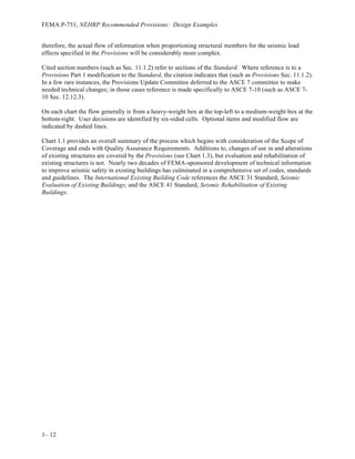
Chart 1.25
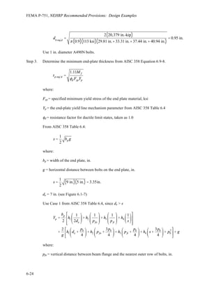
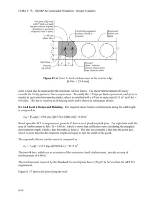
Quality Assurance
Seismic-force-resisting system
assigned to Seismic Design
Category C, D, E, or F? or
Designated seismic system in
structure assigned to Seismic
Design Category D, E, or F?
Satisfy exceptions
in Sec. 11A.1.1?
QA plan not
required.
Registered design professional must
prepare QA plan and affected contractors
must submit statements of responsibility
(Sec. 11A.1.2).
Satisfy testing and
inspection requirements
in the reference standards
(Ch. 13 and 14).
Done.
Reporting and compliance procedures
are given (Sec. 11A.4).
Registered design
professional must perform
structural observations
(Sec. 11A.3).
Occupancy Category III or IV?
or Height 75 ft? or
Seismic Design Category E or F
and more than two stories?
Seismic Design
Category C?
Special inspection is required for some
aspects of the following: deep foundations,
reinforcing steel, concrete, masonry, steel
connections, wood connections, cold-formed
steel connections, selected architectural
components, selected mechanical and
electrical components, isolator units, and
energy dissipation devices (Sec. 11A.1.3).
Special testing is required for some aspects
of the following: reinforcing and prestressing
steel, welded steel, mechanical and electrical
components and mounting systems (Sec. 3.4
[2.4]), and seismic isolation systems
(Sec. 11A.2).
No
Yes
Yes
No
Yes
No
No
Yes](https://image.slidesharecdn.com/femap-751-220509234918-ab6a7ec3/85/FEMA_P-751-pdf-59-320.jpg)


![Chapter 3: Earthquake Ground Motion
3-5
probabilistic ground motions in ASCE 7-05. Consequently, in the WUS the risk-targeted ground motions
in the 2009 Provisions and ASCE 7-10 are generally within 15% of the corresponding uniform-hazard
(2% in 50-year) ground motions. In the Central and Eastern US, where the shapes of hazard curves are
known to differ from those in the WUS, the risk-targeted ground motions generally are smaller. For
instance, in the New Madrid Seismic Zone and near Charleston, South Carolina ratios of risk-targeted to
uniform-hazard ground motions are as small as 0.7.
The computation of risk-targeted probabilistic ground motions for the MCER ground motions in the 2009
Provisions and ASCE 7-10 is detailed in Provisions Part 1 Sections 21.2.1.2 and C21.2.1 and in Luco et
al. (2007). While the computation of the risk-targeted ground motions is different than that of the
uniform-hazard ground motions specified for the MCE ground motions in ASCE 7-05, both begin with
USGS computations of hazard curves. As explained in Section 3.1.1, the uniform-hazard ground motions
simply interpolate the hazard curves for a 2% probability of exceedance in 50 years. In contrast, the risk-
targeted ground motions make use of entire hazard curves. In either case, the end results are probabilistic
spectral response accelerations at 0.2 seconds and 1 second, for 5% of critical damping and the reference
site class.
3.1.2.2 84th
-Percentile Deterministic Ground Motions
For the MCE ground motion maps in ASCE 7-05, recall (from Section 3.1.1) that the underlying
deterministic ground motions are defined as 150% of median spectral response accelerations. As
explained in the FEMA 303 Commentary (p. 296),
Increasing the median ground motion estimates by 50 percent [was] deemed to provide an
appropriate margin and is similar to some deterministic estimates for a large magnitude
characteristic earthquake using ground motion attenuation functions with one standard
deviation. Estimated standard deviations for some active fault sources have been determined to
be higher than 50 percent, but this increase in the median ground motions was considered
reasonable for defining the maximum considered earthquake ground motions for use in design.
For the MCER ground motions in the 2009 Provisions and ASCE 7-10, however, the BSSC decided to
define directly the underlying deterministic ground motions as those at the level of one standard
deviation. More specifically, they are defined as 84th
-percentile ground motions (since it has been widely
observed that ground motions follow lognormal probability distributions). The remainder of the
definition of the deterministic ground motions remains the same as that used for the MCE ground motions
maps in ASCE 7-05. For example, the lower limits of 1.5g and 0.6g described in Section 3.1.1 are
retained.
The USGS applied a simplification specified by the BSSC in computing the 84th
-percentile deterministic
ground motions for the 2009 Provisions and ASCE 7-10. The 84th
-percentile spectral response
accelerations were approximated as 180% of median values. This approximation corresponds to a
logarithmic ground motion standard deviation of approximately 0.6, as demonstrated in the Provisions
Part 1 Section C21.2.2. The computation of deterministic ground motions is further described in
Provisions Part 2 Section C21.2.2.
3.1.2.3 Maximum-Direction Probabilistic and Deterministic Ground Motions
Due to the ground motion attenuation models used by the USGS in computing them5
, overall the MCE
spectral response accelerations in ASCE 7-05 represent the geometric mean of two horizontal components
of ground motion. Most users of ASCE 7-05 are unaware of this fact, particularly since the discussion
notes on the MCE ground motion maps incorrectly state that they represent “the random horizontal
component of ground motion.” For the 2009 Provisions and ASCE 7-10, the BSSC decided that it would
5
See the January/February 1997 Seismological Research Letters “Special Issue on Ground Motion
Attenuation Relations,” Volume 68, Number 1.](https://image.slidesharecdn.com/femap-751-220509234918-ab6a7ec3/85/FEMA_P-751-pdf-89-320.jpg)


![Chapter 4: Structural Analysis
4-27
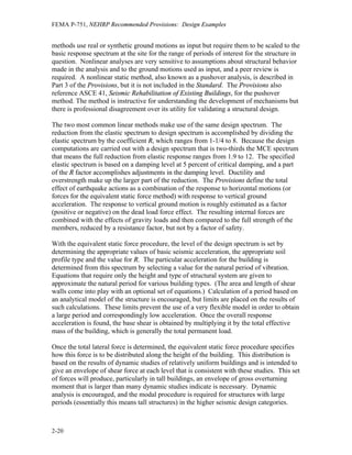
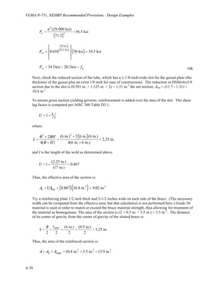
4.1.5.4.3 Setting up the load combinations in SAP2000. The load combinations required for the
analysis are shown in Table 4.1-12.
It should be noted that 32 different load combinations are required only if one wants to maintain the signs
in the member force output, thereby providing complete design envelopes for all members. As mentioned
later, these signs are lost in response spectrum analysis and as a result, it is possible to capture the effects
of dead load plus live load plus-or-minus earthquake load in a single SAP2000 run containing only four
load combinations.
Table 4.1-12 Seismic and Gravity Load Combinations as Run on SAP2000
Run Combination
Lateral* Gravity
A B 1 (Dead) 2 (Live)
One 1 [1] 1.37 0.5
2 [1] 0.73 0.0
3 [7] 1.37 0.5
4 [7] 0.73 0.0
5 [2] 1.37 0.5
6 [2] 0.73 0.0
7 [8] 1.37 0.5
8 [8] 0.73 0.0
Two 1 [3] 1. 37 0.5
2 [3] 0.73 0.0
3 [4] 1. 37 0.5
4 [4] 0.73 0.0
5 [5] 1. 37 0.5
6 [5] 0.73 0.0
7 [6] 1. 37 0.5
8 [6] 0.73 0.0
Three 1 [9] 1. 37 0.5
2 [9] 0.73 0.0
3 [10] 1. 37 0.5
4 [10] 0.73 0.0
5 [15] 1. 37 0.5
6 [15] 0.73 0.0
7 [16] 1. 37 0.5
8 [16] 0.73 0.0
Four 1 [11] 1. 37 0.5
2 [11] 0.73 0.0
3 [12] 1. 37 0.5
4 [12] 0.73 0.0
5 [13] 1. 37 0.5
6 [13] 0.73 0.0
7 [14] 1. 37 0.5
8 [14] 0.73 0.0
*Numbers in brackets [ ] in represent load cases shown in Figure 4.1-8.](https://image.slidesharecdn.com/femap-751-220509234918-ab6a7ec3/85/FEMA_P-751-pdf-139-320.jpg)


![FEMA P-751, NEHRP Recommended Provisions: Design Examples
4-30
The X- and Y-translation periods of 2.87 and 2.60 seconds, respectively, are somewhat longer than the
upper limit on the approximate period, CuTa, of 2.23 seconds.
The first and second mode periods are virtually identical to the periods compute by Rayleigh analysis
(2.85 and 2.56 seconds in the X and Y directions, respectively). The closeness of the Rayleigh and
eigenvalue periods for this building arises from the fact that the first and second modes of vibration act
primarily along the orthogonal axes. Had the first and second modes not acted along the orthogonal axes,
the Rayleigh periods (based on loads and displacements in the X and Y directions) would have been
somewhat less accurate.
Standard Section 12.9.1 specifies that “the analysis shall include a sufficient number of modes to obtain a
combined modal mass participation of at least 90 percent of the total mass in each of the orthogonal
horizontal directions of response considered by the model”. Usually, this is a straightforward requirement
and the first twelve modes would be sufficient for a 12-story building. For this building, however, twelve
modes capture only about 82 percent of the X and Y direction mass. (The effective mass as a fraction of
total mass is shown in brackets [ ] in Columns 3 through 5 of Tables 4.1-13 and 4.1-14.) Most of the
remaining effective mass is in the grade-level slab and in the basement walls. This mass does not show
up until Mode 112 in the Y direction and Mode 118 in the X direction. This is shown in Table 12.1-14,
which provides the periods and effective modal masses in Modes 108 through 119. The intermediate
modes (13 through 107) represent primarily vertical vibration of various portions of the floor diaphragms.
Analyzing the system with 120 or more modes might provide useful information on the response of the
basement level, including shears through the basement and total system base shears at the base of the
basement. However, there would be some difficulty in interpreting the results because the model did not
include sub-grade soil that would be in contact with the basement walls and which would absorb part of
the base shear. Additionally, the computed response of the upper 12 levels of the building, which is the
main focus of this analysis, is virtually identical for the 12 and the 120 mode analyses. For this reason,
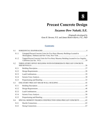
the modal response spectrum analysis discussed in this example was run with only the first 12 modes
listed in Table 4.1-13.
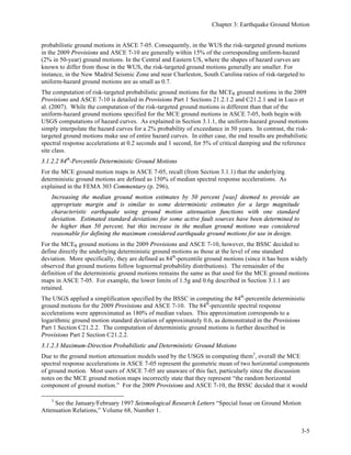
Mode 1: T = 2.87 sec
Mode 2: T = 2.60 sec](https://image.slidesharecdn.com/femap-751-220509234918-ab6a7ec3/85/FEMA_P-751-pdf-142-320.jpg)
![Chapter 4: Structural Analysis
4-31
Mode 3: T = 1.57 sec
Mode 4: T = 1.15 sec
Mode 5: T = 0.98 sec
Mode 6: T = 0.71 sec
Mode 7: T = 0.68 sec Mode 8: T = 0.57 sec
Figure 4.1-10 First eight mode shapes
Table 4.1-13 Computed Periods and Effective Mass Factors (Lower Modes)
Mode
Period
(sec.)
Effective Mass Factor [Accum Mass Factor]
X Translation Y Translation Z Rotation
1 2.87 0.6446 [0.64] 0.0003 [0.00] 0.0028 [0.00]
2 2.60 0.0003 [0.65] 0.6804 [0.68] 0.0162 [0.02]
3 1.57 0.0035 [0.65] 0.0005 [0.68] 0.5806 [0.60]
4 1.15 0.1085 [0.76] 0.0000 [0.68] 0.0000 [0.60]
5 0.975 0.0000 [0.76] 0.0939 [0.78] 0.0180 [0.62]
6 0.705 0.0263 [0.78] 0.0000 [0.78] 0.0271 [0.64]
7 0.682 0.0056 [0.79] 0.0006 [0.79] 0.0687 [0.71]
8 0.573 0.0000 [0.79] 0.0188 [0.79] 0.0123 [0.73]](https://image.slidesharecdn.com/femap-751-220509234918-ab6a7ec3/85/FEMA_P-751-pdf-143-320.jpg)
![FEMA P-751, NEHRP Recommended Provisions: Design Examples
4-32
Table 4.1-13 Computed Periods and Effective Mass Factors (Lower Modes)
Mode
Period
(sec.)
Effective Mass Factor [Accum Mass Factor]
X Translation Y Translation Z Rotation
9 0.434 0.0129 [0.80] 0.0000 [0.79] 0.0084 [0.73]
10 0.387 0.0048 [0.81] 0.0000 [0.79] 0.0191 [0.75]
11 0.339 0.0000 [0.81] 0.0193 [0.81] 0.0010 [0.75]
12 0.300 0.0089 [0.82] 0.0000 [0.81] 0.0003 [0.75]
Table 4.1-14 Computed Periods and Effective Mass Factors (Higher Modes)
Mode
Period
(sec.)
Effective Mass Factor [Accum Effective Mass]
X Translation Y Translation Z Rotation
108 0.0693 0.0000 [0.83] 0.0000 [0.83] 0.0000 [0.79]
109 0.0673 0.0000 [0.83] 0.0000 [0.83] 0.0000 [0.79]
110 0.0671 0.0000 [0.83] 0.0354 [0.86] 0.0000 [0.79]
111 0.0671 0.0000 [0.83] 0.0044 [0.87] 0.0000 [0.79]
112 0.0669 0.0000 [0.83] 0.1045 [0.97] 0.0000 [0.79]
113 0.0663 0.0000 [0.83] 0.0000 [0.97] 0.0000 [0.79]
114 0.0646 0.0000 [0.83] 0.0000 [0.97] 0.0000 [0.79]
115 0.0629 0.0000 [0.83] 0.0000 [0.97] 0.0000 [0.79]
116 0.0621 0.0008 [0.83] 0.0010 [0.97] 0.0000 [0.79]
117 0.0609 0.0014 [0.83] 0.0009 [0.97] 0.0000 [0.79]
118 0.0575 0.1474 [0.98] 0.0000 [0.97] 0.0035 [0.80]
119 0.0566 0.0000 [0.98] 0.0000 [0.97] 0.0000 [0.80]
4.1.6.1 Response spectrum coordinates and computation of modal forces. The coordinates of the
response spectrum are based on Standard Section 11.4.5. This spectrum consists of three parts (for
periods less than TL = 8.0 seconds) as follows:
§ For periods less than T0:
0
0.6 0.4
DS
a DS
S
S T S
T
= +
§ For periods between T0 and TS:
a DS
S S
=
§ For periods greater than TS:
1
D
a
S
S
T
=
where T0 = 0.2SD1/SDS and TS = SD1/SDS.](https://image.slidesharecdn.com/femap-751-220509234918-ab6a7ec3/85/FEMA_P-751-pdf-144-320.jpg)


![FEMA P-751, NEHRP Recommended Provisions: Design Examples
4-40
and difficult aspects of response history approaches. The motions should be characteristic of the site and
should be from real (or simulated) ground motions that have a magnitude, distance and source mechanism
consistent with those that control the maximum considered earthquake (MCE).
For the purposes of this example, however, the emphasis is on the implementation of the response history
approach rather than on selection of realistic ground motions. For this reason, the motion suite developed
for Example 4.2 is also used for the present example.5
The structure for Example 4.2 is situated in
Seattle, Washington and uses three pairs of motions developed specifically for the site. The use of the
Seattle motions for a Stockton building analysis is, of course, not strictly consistent with the requirements
of the Standard. However, a realistic comparison may still be made between the ELF, response spectrum
and response history approaches.
4.1.7.1 The Seattle ground motion suite. It is beneficial to provide some basic information on the
Seattle motion suites in Table 4.1-20a below. Refer to Figures 4.2-40 through 4.2-42 for additional
information, including plots of the ground acceleration histories and 5-percent damped response spectra
for each component of each motion.
The acceleration histories for each source motion were downloaded from the PEER NGA Strong Ground
Motion Database:
http://peer.berkeley.edu/products/strong_ground_motion_db.html
The PEER NGA record number is provided in the first column of the table. Note that the magnitude,
epicenter distance and site class were obtained from the NGA Flatfile (a large Excel file that contains
information about each NGA record).
Table 4.1-20a Suite of Ground Motions Used for Response History Analysis
NGA
Record
Number
Magnitude
[Epicenter
Distance,
km]
Site
Class
Number of
Points and
Digitization
Increment
Component Source
Motion
PGA
(g)
Record
Name
(This
Example)
0879
7.28
C
9625 @
0.005 sec
Landers/LCN260* 0.727 A00
[44] Landers/LCN345* 0.789 A90
0725
6.54
D
2230 @
0.01 sec
SUPERST/B-POE270 0.446 B00
[11.2] SUPERST/B-POE360 0.300 B90
0139
7.35
C
1192 @
0.02 sec
TABAS/DAY-LN 0.328 C00
[21] TABAS/DAY-TR 0.406 C90
*Note that the two components of motion for the Landers earthquake are apparently separated by an
85 degree angle, not 90 degrees as is traditional. It is not known whether these are true orientations or
whether there is an error in the descriptions provided in the NGA database.
Before the ground motions may be used in the response history analysis, they must be scaled for
compatibility with the design spectrum. The scaling procedures for three-dimensional dynamic analysis
are provided in Section 16.1.3.2 of ASCE 7-10. These requirements are provided verbatim as follows:
5
See Sec. 3.2.6.2 of this volume of design examples for a detailed discussion of the selection and scaling of ground motions.](https://image.slidesharecdn.com/femap-751-220509234918-ab6a7ec3/85/FEMA_P-751-pdf-152-320.jpg)


![Chapter 4: Structural Analysis
4-47
The analysis was performed without the (I/R) factor, so in conformance with Section 16.1.4 of
ASCE 7-10, all force quantities produced from the analysis were multiplied by this factor. All
displacements from the analysis were multiplied by the factor Cd/R.
Additionally, the 2010 version of the Standard requires that forces be scaled by the factor 0.85V/Vi where
the base shears from the response history analysis, Vi, are less than 0.85 times the base shears, V,
produced by the ELF method when either Equation 12.8-5 or 12.8-6 controls the seismic base shear. The
displacements must be scaled by the same factor only if Equation 12.8-6 controls when computing the
seismic base shear. (It is noted that these requirements are similar to the scaling requirements provided
for modal response spectrum analysis [Sections 12.9.4.1 and 12.9.4.2] except that forces from modal
response spectrum analysis would be scaled if the shear from the response spectrum analysis is less than
0.85V, regardless of the Cs equation which controls V.)
The base shears from the SS scaled motions with the I/R = 1/8 scaling are provided in the first column of
Table 4.1-22. These forces are all significantly less than 0.85 times the ELF base shear, which is
0.85(112.5) = 956 kips. The required scale factors to bring the base shears up to the 85 percent
requirement are shown in Column 2 of Table 4.2-22.
Before proceeding, it is important to remind the reader that three separate sets of scale factors apply to the
response history analysis of this structure when member design forces are being obtained:
1. The ground motion SS scale factors
2. The I/R scale factor
3. The 0.85V/Vi factor because the base shear from modal response history analysis (including scale
factors 1 and 2 above) is less than 85 percent of that determined from ELF when ELF is governed
by Equation 12.8-5 or 12.8-6.
Table 4.1-22 I/R Scaled Shears and Required 85% Rule Scale Factors
Analysis
(I/R) times maximum base
shear from analysis
(kips)
Required additional scale factor for
V = 0.85VELF = 956 kips
A00-X 438.4 2.18
A00-Y 446.7 2.14
A90-X 198.5 4.81
A90-Y 173.9 5.49
B00-X 376.1 2.54
B00-Y 391.2 2.44
B90-X 364.8 2.62
B90-Y 432.5 2.21
C00-X 391.2 2.44
C00-Y 300.9 3.18
C90-X 403.6 2.37
C90-Y 634.4 1.51
1.0 kip = 4.45 kN](https://image.slidesharecdn.com/femap-751-220509234918-ab6a7ec3/85/FEMA_P-751-pdf-159-320.jpg)


![Chapter 4: Structural Analysis
4-71
Columns hinge only at the base and the plastic moment capacity is assumed to be Zcol(Fye-Pu/Acol). The
fully plastic mechanism for the system is illustrated in Figure 4.2-6. The inset to the figure shows how
the angle modification term, σ, was computed. The strength, V, for the total structure is computed from
the following relationships (see Figure 4.2-6 for nomenclature):
§ Internal Work = External Work
§ Internal Work = 2[20σθMPA + 40σθMPB + θ(MPC + 4MPD + MPE)]
§
1 1
External Work = where 1
nLevels nLevels
i i i
i i
V F H F
θ
= =
=
∑ ∑
Three lateral force patterns are used: uniform, upper triangular and Standard (where the Standard pattern
is consistent with the vertical force distribution of Table 4.2-3 in this volume of design examples). The
results of the analysis are shown in Table 4.2-7. As expected, the strength under uniform load is
significantly greater than under triangular or Standard load. The closeness of the Standard and triangular
load strengths results from the vertical-load-distributing parameter (k = 1.385) being close to 1.0.
The ELF base shear, 759 kips (see Table 4.2-3), when divided by the Standard pattern capacity,
2,616 kips, is 0.29. This is reasonably consistent with the DCRs shown in Figure 4.2-5.
Table 4.2-7 Lateral Strength on Basis of Rigid-Plastic Mechanism
Lateral Load Pattern
Lateral strength for
entire structure (kips)
Lateral strength
single frame (kips)
Uniform 3,332 1,666
Upper Triangular 2,747 1,373
Standard 2,616 1,308](https://image.slidesharecdn.com/femap-751-220509234918-ab6a7ec3/85/FEMA_P-751-pdf-183-320.jpg)


![FEMA P-751, NEHRP Recommended Provisions: Design Examples
4-96
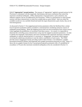
included through the use of the outrigger column shown at the right of Figure 4.2-4. Figure 4.2-26 plots
two base shear components of the pushover response for the SP structure subjected to the ML loading.
Also shown is the total response. The kink in the line representing P-delta forces occurs because these
forces are based on first-story displacement, which, for an inelastic system, generally will not be
proportional to the roof displacement.
For all of the pushover analyses reported in this example, the structure is pushed to a displacement of
37.5 inches at the roof level. This value is approximately 4 percent of the total height.
Figure 4.2-26 Two base shear components of pushover response
4.2.5.1 Pushover response of strong panel structure. Figure 4.2-27 shows the pushover response of
the SP structure to all three lateral load patterns where P-delta effects are excluded. In each case, gravity
loads are applied first, and then the lateral loads are applied using the displacement control algorithm.
Figure 4.2-28 shows the response curves if P-delta effects are included. In Figure 4.2-29, the response of
the structure under ML loading with and without P-delta effects is illustrated. Clearly, P-delta effects are
an extremely important aspect of the response of this structure and the influence grows in significance
after yielding. This is particularly interesting in the light of the Standard, which ignores P-delta effects in
elastic analysis if the maximum stability ratio is less than 0.10 (see Sec. 12.8-7). For this structure, the
maximum computed stability ratio is 0.0862 (see Table 4.2-5), which is less than 0.10 and is also less
than the upper limit of 0.0909. The upper limit is computed according to Standard Equation 12.8-17 and
is based on the very conservative assumption that β = 1.0. While the Standard allows the analyst to
exclude P-delta effects in an elastic analysis, this clearly should not be done in the pushover analysis (or
in response history analysis). (In the Provisions the upper limit for the stability ratio is eliminated.
Where the calculated θ is greater than 0.10, a pushover analysis must be performed in accordance with
ASCE 41, and it must be shown that that the slope of the pushover curve is positive up to the target
displacement. The pushover analysis must be based on the MCE spectral acceleration and must include
P-delta effects [and loss of strength, as appropriate]. If the slope of the pushover curve is negative at
displacements less than the target displacement, the structure must be redesigned such that θ is less than
0.10 or the pushover slope is positive up to the target displacement.)
-1,000
0
1,000
2,000
0 10 20 30 40
S
h
e
a
r
(
k
i
p
s
)
Roof displacement (inches)
Column shearforces
Totalbase shear
P-Delta forces](https://image.slidesharecdn.com/femap-751-220509234918-ab6a7ec3/85/FEMA_P-751-pdf-208-320.jpg)


![Chapter 5: Foundation Analysis and Design
5-5
Table 5.1-1 Geotechnical Parameters
Parameter Value
Net bearing pressure (to control
settlement due to sustained loads)
≤ 4,000 psf for B ≤ 20 feet
≤ 2,000 psf for B ≥ 40 feet
(may interpolate for intermediate dimensions)
Bearing capacity (for plastic
equilibrium strength checks with
factored loads)
2,000B psf for concentrically loaded square footings
3,000B' psf for eccentrically loaded footings
where B and B' are in feet, B is the footing width and B' is
an average width for the compressed area.
Resistance factor, φ = 0.7
[This φ factor for cohesionless soil is specified in
Provisions Part 3 Resource Paper 4; the value is set at 0.7
for vertical, lateral and rocking resistance.]
Lateral properties
Earth pressure coefficients:
§ Active, KA = 0.3
§ At-rest, K0 = 0.46
§ Passive, KP = 3.3
“Ultimate” friction coefficient at base of footing = 0.65
Resistance factor, φ = 0.7
The structural material properties assumed for this example are as follows:
§ f'c = 4,000 psi
§ fy = 60,000 psi
5.1.1.2 Seismic Parameters. The complete set of parameters used in applying the Provisions to design of
the superstructure is described in Section 6.2.2.1 of this volume of design examples. The following
parameters, which are used during foundation design, are duplicated here.
§ Site Class = D
§ SDS = 1.0
§ Seismic Design Category = D](https://image.slidesharecdn.com/femap-751-220509234918-ab6a7ec3/85/FEMA_P-751-pdf-253-320.jpg)


![Chapter 5: Foundation Analysis and Design
5-9
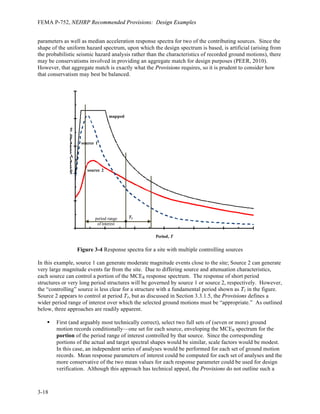
For use in subsequent calculations, the factored bearing pressure qu = 621 kips/(11 ft)2
= 5.13 ksf.
5.1.2.3 Footing Thickness. Once the plan dimensions of the footing are selected, the thickness is
determined such that the section satisfies the one-way and two-way shear demands without the addition of
shear reinforcement. Demands are calculated at critical sections, shown in Figure 5.1-2, which depend on
the footing thickness.
Check a footing that is 26 inches thick:
For the W14 columns used in this building, the side dimensions of the loaded area (taken halfway
between the face of the column and the edge of the base plate) are approximately 16 inches.
Accounting for cover and expected bar sizes, d = 26 - (3 + 1.5(1)) = 21.5 in.
One-way shear:
( )
16
12
11 21.5
11 5.13
2 12
u
V
⎛ ⎞
−
= −
⎜ ⎟
⎝ ⎠
= 172 kips
( ) ( )( )( )
1
1,000
0.75 2 4,000 11 12 21.5
n c
V V
φ φ
= = × = 269 kips 172 kips OK
Two-way shear:
( ) ( )
2
16 21.5
12
621 5.13
u
V +
= − = 571 kips
( ) ( ) ( )( )
1
1,000
0.75 4 4,000 4 16 21.5 21.5
n c
V V
φ φ ⎡ ⎤
= = × +
⎣ ⎦ = 612 kips 571 kips OK
5.1.2.4 Footing Reinforcement. Footing reinforcement is selected considering both flexural demands
and minimum reinforcement requirements. The following calculations treat flexure first because it
usually controls:
( ) ( )
2
16
12
11
1
11 5.13 659 ft-kips
2 2
u
M
⎛ ⎞
−
= =
⎜ ⎟
⎝ ⎠
Try nine #8 bars each way. The distance from the extreme compression fiber to the center of the top layer
of reinforcement, d = t - cover - 1.5db = 26 - 3 - 1.5(1) = 21.5 in.
T = As fy = 9(0.79)(60) = 427 kips
Noting that C = T and solving the expression C = 0.85 f'c b a for a produces a = 0.951 in.
( ) ( )( )( )
0.951 1
2 2 12
0.90 427 21.5
a
n
M T d
φ φ
= − = − = 673 ft-kips 659 ft-kips OK
The ratio of reinforcement provided is ρ = 9(0.79)/[(11)(12)(26)] = 0.00207. The distance between bars
spaced uniformly across the width of the footing is s = [(11)(12)-2(3+0.5)]/(9-1) = 15.6 in.
According to ACI 318 Section 7.12, the minimum reinforcement ratio = 0.0018 0.00207 OK](https://image.slidesharecdn.com/femap-751-220509234918-ab6a7ec3/85/FEMA_P-751-pdf-257-320.jpg)


![Chapter 5: Foundation Analysis and Design
5-13
Section 6.2.3.5 of this volume of design examples outlines the design load combinations, which include
the redundancy factor as appropriate. A large number of load cases result from considering two senses of
accidental torsion for loading in each direction and including orthogonal effects . The detailed
calculations presented here are limited to two primary conditions, both for a combined foundation for
columns at Grids A-5 and A-6: the downward case (1.4D + 0.5L + 0.3Ex + 1.0Ey) and the upward case
(0.7D + 0.3Ex + 1.0Ey).
Before loads can be computed, attention must be given to Standard Section 12.13.4. That Section states
that “overturning effects at the soil-foundation interface are permitted to be reduced by 25 percent” where
the ELF procedure is used and by 10 percent where modal response spectrum analysis is used. Because
the overturning effect in question relates to the global overturning moment for the system, judgment must
be used in determining which design actions may be reduced. If the seismic force-resisting system
consists of isolated shear walls, the shear wall overturning moment at the base best fits that description.
For a perimeter moment-resisting frame, most of the global overturning resistance is related to axial loads
in columns. Therefore, in this example column axial loads (Fz) from load cases Ex and Ey are multiplied
by 0.75 and all other load effects remain unreduced.
5.1.3.2 Downward Case (1.4D + 0.5L + 0.3Ex + 1.0Ey). In order to perform the overturning checks, a
footing size must be assumed. Preliminary checks (not shown here) confirmed that isolated footings
under single columns were untenable. Check overturning for a footing that is 9 feet wide by 40 feet long
by 5 feet thick. Furthermore, assume that the top of the footing is 2 feet below grade (the overlying soil
contributes to the resisting moment). (In these calculations the 0.2SDSD modifier for vertical accelerations
is used for the dead loads applied to the foundation but not for the weight of the foundation and soil. This
is the author’s interpretation of the Standard. The footing and soil overburden are not subject to the same
potential for dynamic amplification as the dead load of the superstructure and it is not common practice to
include the vertical acceleration on the weight of the footing and the overburden. Furthermore, for
footings that resist significant overturning, this issue makes a significant difference in design.)
Combining the loads from columns at Grids A-5 and A-6 and including the weight of the foundation and
overlying soil produces the following loads at the foundation-soil interface:
P = applied loads + weight of foundation and soil
= 1.4(-203.8 - 103.5) + 0.5(-43.8 - 22.3) +0.75[0.3(3.8 + 51.8) + 1.0(-21.3 + 281)]
- 1.2[9(40)(5)(0.15) + 9(40)(2)(0.125)]
= -688 kips.
Mxx = direct moments + moment due to eccentricity of applied axial loads
= 0.3(53.6 + 47.7) + 1.0(-1011.5 - 891.0)
+ [1.4(-203.8) + 0.5(-43.8) + 0.75(0.3)(3.8) + 0.75(1.0)(-21.3)](12.5)
+ [1.4(-103.5) + 0.5(-22.3) + 0.75(0.3)(51.8) + 0.75(1.0)(281)](-12.5)
= -6,717 ft-kips.
Myy = 0.3(-243.1 - 246.9) + 1.0(8.1 + 13.4)
= -126 ft-kips. (The resulting eccentricity is small enough to neglect here, which simplifies the
problem considerably.)
Vx = 0.3(-13.8 - 14.1) + 1.0(0.5 + 0.8)
= -7.11 kips.
Vy = 0.3(4.6 + 3.7) + 1.0(-85.1 -68.2)
= -149.2 kips.](https://image.slidesharecdn.com/femap-751-220509234918-ab6a7ec3/85/FEMA_P-751-pdf-261-320.jpg)


![Chapter 5: Foundation Analysis and Design
5-39
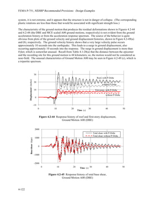
Figure 5.2-13 P-M interaction diagram for Site Class E
5.2.2.4 Pile Length for Axial Loads. For the calculations that follow, recall that skin friction and end
bearing are neglected for the top 3 feet in this example. The design is based on having 1’-6” of soil over a
4’-0” deep pile cap.
5.2.2.4.1 Length for Settlement. Service loads per pile are calculated as P = (PD + PL)/4.
Check the pile group under the side column in Site Class C, assuming L = 52.5 feet – 5.5 feet = 47 feet:
P = (752 + 114)/4 = 217 kips.
Pskin = average friction capacity × pile perimeter × pile length for friction
= 0.5[0.3 + 2.5(0.03) + 0.3 + 49.5(0.03)]π(22/12)(44) = 292 kips
Pend = end bearing capacity at depth × end bearing area
= [65 + 49.5(0.6)](π/4)(22/12)2
= 250 kips
Pallow = (Pskin + Pend)/S.F. = (292 + 250)/2.5 = 217 kips = 217 kips (demand) OK
Check the pile group under the corner column in Site Class E, assuming L = 49 feet:
P = (460 + 77)/4 = 134 kips
-300
-200
-100
0
100
200
300
400
500
600
700
800
0 500 1000 1500 2000 2500
A
x
i
a
l
l
o
a
d
,
P
(
k
i
p
)
Moment, M (in.-kip)
8-#7
8-#6
6-#6
6-#5
Side
Corner](https://image.slidesharecdn.com/femap-751-220509234918-ab6a7ec3/85/FEMA_P-751-pdf-287-320.jpg)
![FEMA P-751, NEHRP Recommended Provisions: Design Examples
5-40
Pskin = [friction capacity in first layer + average friction capacity in second layer] × pile perimeter
= [24.5(0.3) + (24.5/2)(0.9 + 0.9 + 24.5[0.025])]π(22/12) = 212 kips
Pend = [40 + 24.5(0.5)](π/4)(22/12)2
= 138 kips
Pallow = (212 + 138)/2.5 = 140 kips 134 kips OK
5.2.2.4.2 Length for Compression Capacity. All of the strength-level load combinations (discussed in
Section 5.2.1.3) must be considered.
Check the pile group under the side column in Site Class C, assuming L = 49 feet:
As seen in Figure 5.1-12, the maximum compression demand for this condition is Pu = 394 kips.
Pskin = 0.5[0.3 + 0.3 + 47(0.03)]π(22/12)(47) = 272 kips
Pend = [65 + 47(0.6)](π/4)(22/12)2
= 246 kips
φPn = φ(Pskin + Pend) = 0.75(272 + 246) = 389 kips ≈ 390 kips OK
Check the pile group under the corner column in Site Class E, assuming L = 64 feet:
As seen in Figure 5.2-13, the maximum compression demand for this condition is Pu = 340 kips.
Pskin = [27(0.3) + (34/2)(0.9 + 0.9 + 34[0.025])]π(22/12) = 306 kips
Pend = [40 + 34(0.5)](π/4)(22/12)2
= 150 kips
φPn = φ(Pskin + Pend) = 0.75(306 + 150) = 342 kips 340 kips OK
5.2.2.4.3 Length for Uplift Capacity. Again, all of the strength-level load combinations (discussed in
Section 5.2.1.3) must be considered.
Check the pile group under side column in Site Class C, assuming L = 5 feet:
As seen in Figure 5.2-12, the maximum tension demand for this condition is Pu = -1.9 kips.
Pskin = 0.5[0.3 + 0.3 + 2(0.03)]π(22/12)(2) = 3.8 kips
φPn = φ(Pskin) = 0.75(3.8) = 2.9 kips 1.9 kips OK
Check the pile group under the corner column in Site Class E, assuming L = 52 feet:
As seen in Figure 5.2-13, the maximum tension demand for this condition is Pu = -144 kips.
Pskin = [27(0.3) + (22/2)(0.9 + 0.9 + 22[0.025])]π(22/12) = 196 kips
φPn = φ(Pskin) = 0.75(196) = 147 kips 144 kips OK](https://image.slidesharecdn.com/femap-751-220509234918-ab6a7ec3/85/FEMA_P-751-pdf-288-320.jpg)


![Chapter 5: Foundation Analysis and Design
5-47
Figure 5.2-16 being unreinforced would satisfy the Provisions requirements, but the author has decided to
extend very light longitudinal and nominal transverse reinforcement for the full length of the pile.
5.2.3 Other
Considerations
5.2.3.1 Foundation Tie Design and Detailing. Standard Section 12.13.5.2 requires that individual pile
caps be connected by ties. Such ties are often grade beams, but the Standard would permit use of a slab
(thickened or not) or calculations that demonstrate that the site soils (assigned to Site Class A, B, or C)
provide equivalent restraint. For this example, a tie beam between the pile caps under a corner column
and a side column is designed. The resulting section is shown in Figure 5.2-18.
For pile caps with an assumed center-to-center spacing of 32 feet in each direction and given Pgroup =
1,224 kips under a side column and Pgroup = 1,142 kips under a corner column, the tie is designed as
follows.
As indicated in Standard Section 12.13.5.2, the minimum tie force in tension or compression equals the
product of the larger column load times SDS divided by 10 = 1224(1.1)/10 = 135 kips.
The design strength for six #6 bars is as follows
φAs fy = 0.9(6)(0.44)(60) = 143 kips 135 kips OK
According to ACI 318 Section 21.12.3.2, the smallest cross-sectional dimension of the tie beam must not
be less than the clear spacing between pile caps divided by 20 = (32'-0 - 9'-2)/20 = 13.7 inches. Use a
tie beam that is 14 inches wide and 16 inches deep. ACI 318 Section 21.12.3.2 further indicates that
closed ties must be provided at a spacing of not more than one-half the minimum dimension, which is
14/2 = 7 inches.
Assuming that the surrounding soil provides restraint against buckling, the design strength of the tie beam
concentrically loaded in compression is as follows:
φPn = 0.8φ[0.85f'c(Ag - Ast) + fyAst]
= 0.8(0.65)[0.85(3){(16)(14) – 6(0.44)}+ 60(6)(0.44)] = 376 kips 135 kips OK
Figure 5.2-18 Foundation tie section
(3) #6 top bars
(3) #6 bottom bars
#4 ties at 7 o.c.
2 clear
at sides
3 clear at
top and bottom](https://image.slidesharecdn.com/femap-751-220509234918-ab6a7ec3/85/FEMA_P-751-pdf-295-320.jpg)


![FEMA P-751, NEHRP Recommended Provisions: Design Examples
5-50
The engineering framework established in ASCE 41 is more conducive to explicit use of performance
measures. In that document (Sections 4.4.3.2.1 and 4.4.3.3.1), the use of fixed-based structural models is
prohibited for “buildings being rehabilitated for the Immediate Occupancy Performance Level that are
sensitive to base rotations or other types of foundation movement.” In this case the focus is on damage
control rather than structural stability.
5.2.3.5.2 Example Calculations. To assess the significance of foundation flexibility, one may compare
the dynamic characteristics of a fixed-base model to those of a model in which foundation effects are
included. The effects of foundation flexibility become more pronounced as foundation period and
structural period approach the same value. For this portion of the example, use the Site Class E pile
design results from Section 5.2.2.1 and consider the north-south response of the concrete moment frame
building located in Berkeley (Section 7.2) as representative for this building.
5.2.3.5.2.1 Stiffness of the Structure. Calculations of the effect of foundation flexibility on the dynamic
response of a structure should reflect the overall stiffness of the structure (e.g., that associated with the
fundamental mode of vibration) rather than the stiffness of any particular story. Table 7-2 shows that the
total weight of the structure is 43,919 kips. Table 7-3 shows that the calculated period of the fixed-base
structure is 2.02 seconds and Table 7-7 indicates that 83.6 percent of the mass participates in that mode.
Using the equation for the undamped period of vibration of a single-degree-of-freedom oscillator, the
effective stiffness of the structure is as follows:
( )
2
2
2 2
4 (0.836)43,919 386.1
4
920 kip/in.
2.02
M
K
T
π
π
= = =
5.2.3.5.2.2 Foundation Stiffness. As seen in Figure 7-1, there are 36 moment frame columns. Assume
that a 2×2 pile group supports each column. As shown in Section 5.2.2.1, the stiffness of each pile is
40 kip/in. Neglecting both the stiffness contribution from passive pressure resistance and the flexibility
of the beam-slab system that ties the pile caps, the stiffness of each pile group is 4 × 40 = 160 kip/in. and
the stiffness of the entire foundation system is 36 × 160 = 5,760 kip/in.
5.2.3.5.2.3 Effect of Foundation Flexibility. Because the foundation stiffness is much greater than the
structural stiffness, period elongation is expected to be minimal. To confirm this expectation, the period
of the combined system is computed. The total stiffness for the system (springs in series) is as follows:
1 1
793 kip/in.
1 1 1 1
920 5760
combined
structure fdn
K
K K
= = =
+ +
Assume that the weight of the foundation system is 4,000 kips and that 100 percent of the corresponding
mass participates in the new fundamental mode of vibration. The period of the combined system is as
follows:
[ ]
(0.836)(43,919) (1.0)(4000) 386.1
2 2 2.29 sec
793
M
T
K
π π
+
= = =
which is an increase of 13 percent over that predicted by the fixed-base model. For systems responding in
the constant-velocity portion of the spectrum, accelerations (and thus forces) are a function of 1/T and
relative displacements are a function of T. Therefore, with respect to the fixed-based model, the](https://image.slidesharecdn.com/femap-751-220509234918-ab6a7ec3/85/FEMA_P-751-pdf-298-320.jpg)


![Chapter 6: Structural Steel Design
6-51
The column-beam strength ratio calculation is illustrated for the lower level in the E-W direction,
Level 2, at Gridline D (W24x146 column and W21x73 beam).
For the beams:
2 2
c c
pb pr e h g h
d d
M M V S V S
⎛ ⎞ ⎛ ⎞
= + + ± +
⎜ ⎟ ⎜ ⎟
⎝ ⎠ ⎝ ⎠
where:
Mpr = CprRyFy Ze = (1.15)(1.1)(50) (122) = 7,361 in.-kips
Ry = 1.1 for Grade 50 steel
Ze = Zx -2ctbf (d - tbf) = 172 – 2(1.659)(0.74)(21.24-0.74) = 122 in.3
Sh = Distance from column face to centerline of plastic hinge (see Figure 6.2-9) = a + b/2 = 13.2 in.
for the RBS
'
2 /
e pr
V M L
= '
/ 2
g u
V w L
=
L’ = Distance between plastic hinges = 248.8 in.
wu = Factored uniform gravity load along beam
= 1.4D + 0.5L = 1.4[(0.068 ksf)(12.5 ft)+(0.025)(13.3 ft)] + 0.5(0.050 ksf)(12.5 ft)
= 2.42 klf](https://image.slidesharecdn.com/femap-751-220509234918-ab6a7ec3/85/FEMA_P-751-pdf-351-320.jpg)


![FEMA P-751, NEHRP Recommended Provisions: Design Examples
6-80
The maximum allowable value of story drifts summed to the roof of the ten-story hospital building
(156 feet) obtained from an elastic analysis is 18.72 inches. This same figure extracted from a nonlinear
response history analysis cannot exceed 1.25(18.72 in.) = 23.40 in.
6.3.3.6 Seismic weight. The area of the tower floorplate is approximately equal to [(3)(30 ft) +
(2)(8 in.)(1 ft/12 in.)]2
= 8,342 ft2
, while the area of the podium floorplate is approximately [(7)(30 ft) +
(2)(8 in.)(1 ft/12 in.)] × [(4)(30 ft) + (2)(8 in.)(1 ft/12 in.)] = 25,642 ft2
. Thus, the weights that contribute
to seismic forces are as follows:
§ Tower roof:
Roof D = (0.135)(8,342) = 1,126 kips
Cladding = (4)(3)(30)(0.300) = 108 kips
Total = 1,234 kips
§ Tower floor:
Floor D = (0.104)(8,342) = 868 kips
Partitions = (0.010)(8,342) = 83 kips
Cladding = (4)(3)(30)(0.300) = 108 kips
Total = 1,059 kips
§ Podium roof:
Roof D = (0.135)(25,642 - 8,342) = 2,336 kips
Floor D = (0.104)(8,342) = 868 kips
Partitions = (0.010)(8,342) = 83 kips
Cladding = (2)(11)(30)(0.300) = 198 kips
Total = 3,485 kips
§ Podium floor:
Floor D = (0.104)(25,642) = 2,667 kips
Partitions = (0.010)(25,642) = 256 kips
Cladding = (2)(11)(30)(0.300) = 198 kips
Total = 3,121 kips
Total effective seismic weight of building = 1,234 + 7(1,059) + 3,485 + 3,121 = 15,253 kips
6.3.4 Elastic
Analysis
The base shear is determined using an ELF analysis; the base shear so computed is needed later when
evaluating the scaling of the base shears obtained from the modal response spectrum analysis.
In a subsequent section (Section 6.3.6.3.3), columns are designed using forces obtained from nonlinear
response history analyses that are intended to represent the maximum force that can develop in these
elements per the exception to Standard Section 12.4.3.1. Compliance with story drift limits is also
evaluated using the results of the nonlinear response history analyses.](https://image.slidesharecdn.com/femap-751-220509234918-ab6a7ec3/85/FEMA_P-751-pdf-382-320.jpg)


![FEMA P-751, NEHRP Recommended Provisions: Design Examples
7 – 32
Table 7-14b P-Delta Computations for the Honolulu Building Loaded in the E-W Direction
Story
Story Drift
(in)
Story Shear
(kips)
Story Dead
Load (kips)
Story Live
Load (kips)
Total Story
Load (kips)
Accum. Story
Load (kips)
Stability
Coeff, θ
Roof 0.230 177.8 3,352 420 3,772 3,772 0.0079
12 0.376 343.6 3,675 420 4,095 7,867 0.0128
11 0.518 482.5 3,675 420 4,095 11,962 0.0183
10 0.639 596.9 3,675 420 4,095 16,057 0.0239
9 0.736 688.9 3,675 420 4,095 20,152 0.0296
8 0.814 761.0 3,675 420 4,095 24,247 0.0351
7 0.874 815.5 3,675 420 4,095 28,342 0.0407
6 0.915 854.8 3,675 420 4,095 32,437 0.0462
5 0.942 881.2 3,675 420 4,095 36,532 0.0515
4 0.958 897.3 3,675 420 4,095 40,627 0.0568
3 0.970 905.5 3,675 420 4,095 44,722 0.0626
2 1.173 908.5 3,817 420 4,237 48,959 0.0617
(1.0 in = 25.4 mm, 1.0 kip = 4.45 kN)
The stability ratio at Story 5 from Table 7-14b is computed as follows:
Amplified story drift = Δ5 = 0.942 inch
Story shear = V5 = 881.2 = kips
Accumulated story weight P5 = 36,532 kips
Story height = hs5 = 156 inches
Cd = 4.5
θ = [P5 (Δ5/Cd)]/(V5hs5) = 36,532(0.942/4.5)/(881.2)(156) = 0.0515
The requirements for maximum stability ratio (0.5/Cd = 0.5/4.5 = 0.111) are satisfied. Because the
stability ratio is less than 0.10 at all floors, P-delta effects need not be considered (Standard
Section 12.8.7).](https://image.slidesharecdn.com/femap-751-220509234918-ab6a7ec3/85/FEMA_P-751-pdf-454-320.jpg)


![Chapter 7: Reinforced Concrete
7 – 39
Figure 7-10 Layout for beam reinforcement
(1.0 ft = 0.3048 m, 1.0 in. = 25.4 mm)
Given Figure 7-10, compute the effective depth for both positive and negative moment as follows:
Beams spanning in the E-W direction, d = 32 - 1.5 - 0.5 - 1.00/2 = 29.5 inches
Beams spanning in the N-S direction, d = 32 - 1.5 - 0.5 - 1.0 - 1.00/2 = 28.5 inches
For negative moment bending, the effective width is 24 inches for all beams. For positive moment, the
slab is in compression and the effective T-beam width varies according to ACI 318 Section 8.12. The
effective widths for positive moment are as follows (with the parameter controlling effective width shown
in parentheses):
20-foot beams in Frames 1 and 8: b = 24 + 20(12)/12 = 44 inches (span length)
20-foot beams in Frames 2 and 7: b = 20(12)/4 = 60 inches (span length)
40-foot beams in Frames 2 through 7: b = 24 + 2[8(4)] = 88 inches (slab thickness)
30-foot beams in Frames A and D: b = 24 + [6(4)] = 48 inches (slab thickness)
30-foot beams in Frames B and C: b = 24 + 2[8(4)] = 88 inches (slab thickness)
ACI 318 Section 21.5.2 controls the longitudinal reinforcement requirements for beams. The minimum
reinforcement to be provided at the top and bottom of any section is as follows:
2
,
200 200(24)(29.5)
2.36 in
60,000
w
s min
y
b d
A
f
= = =
30
1.5 cover
#8 bar
#4 hoop
East-west
spanning beam
32
29.5
28.5
North-south
spanning beam
B
Column](https://image.slidesharecdn.com/femap-751-220509234918-ab6a7ec3/85/FEMA_P-751-pdf-464-320.jpg)


![FEMA P-751, NEHRP Recommended Provisions: Design Examples
7 – 42
7.4.2.2.1 Longitudinal Reinforcement. The design process for determining longitudinal reinforcement
is illustrated as follows for Span A-A’.
1. Design for Negative Moment at the Face of the Exterior Support (Grid A):
Mu = 1.42(-550) + 0.5(-251) + 1.0(-3,383) = -4,290 inch-kips
Try one #8 bar in addition to the three #8 bars required for minimum steel:
As = 4(0.79) = 3.16 in2
fc' = 5,000 psi
fy = 60 ksi
Width b for negative moment = 24 inches
d = 29.5 in.
Depth of compression block, a = Asfy/0.85fc'b
a = 3.16 (60)/[0.85 (5) 24] = 1.86 inches
Design strength, φ Mn = φ Asfy(d - a/2)
φ Mn = 0.9(3.16)60(29.5 – 1.86/2) = 4,875 inch-kips 4,290 inch-kips OK
2. Design for Positive Moment at Face of Exterior Support (Grid A):
Mu = [-0.68(550)] + [1.0(3,383)] = 3,008 inch-kips
Try the three #8 bars required for minimum steel:
As = [3(0.79)] = 2.37 in 2
Width b for positive moment = 44 inches
d = 29.5 inches
a = [2.37(60)]/[0.85(5)44] = 0.76 inch
φ Mn = 0.9(2.37) 60(29.5 – 0.76/2) = 3,727 inch-kips 3,008 inch-kips OK
3. Positive Moment at Midspan:
Mu = [1.2(474)] + [1.6(218)] = 918.1 inch-kips
Minimum reinforcement (three #8 bars) controls by inspection.
4. Design for Negative Moment at the Face of the Interior Support (Grid A’):
Mu = 1.42(-602) + 0.5(-278) + 1.0(-3,177) = -4,172 inch-kips
Try one #8 bars in addition to the three #8 bars required for minimum steel:
φ Mn = 4,875 inch-kips 4,172 inch-kips OK
5. Design for Positive Moment at Face of Interior Support (Grid A’):
Mu = [-0.68(602)] + [1.0(3,177)] = 2,767 inch-kips
Three #8 bars similar to the exterior support location are adequate by inspection.](https://image.slidesharecdn.com/femap-751-220509234918-ab6a7ec3/85/FEMA_P-751-pdf-467-320.jpg)

![FEMA P-751, NEHRP Recommended Provisions: Design Examples
7 – 44
Table 7-16 Design and Maximum Probable Flexural Strength For Beams in Frame 1
Item
Location*
A A' B C C' D
Negative
Moment
Moment Demand
(inch-kips)
4,290 4,672 4,664 4,664 4,672 4,290
Reinforcement four #8 four #8 four #8 four #8 four #8 four #8
Design Strength
(inch-kips)
4,875 4,875 4,875 4,875 4,875 4,875
Probable Strength
(inch-kips)
7,042 7,042 7,042 7,042 7,042 7,042
Positive
Moment
Moment Demand
(inch-kips)
3,009 3,288 3,255 3,255 3,289 3,009
Reinforcement three #8 three #8 three #8 three #8 three #8 three #8
Design Strength
(inch-kips)
3,727 3,727 3,727 3,727 3,727 3,727
Probable Strength
(inch-kips)
5,159 5,159 5,159 5,159 5,159 5,159
*Moment demand is taken as the larger of the beam moments on each side of the column.
(1.0 in-kip = 0.113 kN-m)
As an example of computation of probable strength, consider the case of four #8 top bars plus the portion
of slab reinforcing within the effective beam flange width computed above, which is assumed to be
0.002(4 inches)(44-24)=0.16 square inches. (The slab reinforcing, which is not part of this example, is
assumed to be 0.002 for minimum steel.)
As = 4(0.79) + 0.16 = 3.32 in2
Width b for negative moment = 24 inches
d = 29.5 inches
Depth of compression block, a = As(1.25fy)/0.85fc'b
a = 3.32(1.25)60/[0.85(4)24] = 2.44 inches
Mpr = 1.0As(1.25fy)(d - a/2)
Mpr = 1.0(3.32)1.25(60)(29.6 – 2.44/2) = 7,042 inch-kips
For the case of three #8 bottom bars:
As = 3(0.79) = 2.37 in2
Width b for positive moment = 44 inches
d = 29.5 inches
a = 2.37(1.25)60/[0.85(5)44] = 0.95 inch
Mpr = 1.0(2.37)1.25(60)(29.5 – 0.95/2) = 5,159 inch-kips
At this point in the design process, the layout of reinforcement has been considered preliminary because
the quantity of reinforcement placed in the beams has a direct impact on the magnitude of the stresses
developed in the beam-column joint. If the computed joint stresses are too high, the only remedies are
increasing the concrete strength, increasing the column area, changing the reinforcement layout, or](https://image.slidesharecdn.com/femap-751-220509234918-ab6a7ec3/85/FEMA_P-751-pdf-469-320.jpg)


(29.5/91.4) = 11.6 inches
15 64 41
φVs = 151.7 kips
(4) Legs, s = 7
91.4 kips
24.8 kips
91.4 kips
24.8 kips
B C
φVs = 79.5 kips
(2) Legs, s = 7](https://image.slidesharecdn.com/femap-751-220509234918-ab6a7ec3/85/FEMA_P-751-pdf-475-320.jpg)
(29.5/58.1) = 9.13 inches
In terms of detailing requirements, ACI 318 Section 21.5.3.1 states that closed hoops at a tighter spacing
are required over a distance of twice the member depth from the face of the support and ACI 318
Section 21.5.3.4 indicates that stirrups are permitted away from the ends.
Therefore, the shear strength requirements at this transition point should be computed. At a point equal to
twice the beam depth, or 64 inches from the support, the shear is computed as:
Vu = 91.4 - (64/210)(91.4 – 24.8) = 71.1 kips
Compute the required spacing assuming two #4 vertical legs:
s = 0.75[2(0.2)](60)(29.5/71.1) = 7.4 inches
Before the final layout can be determined, the detailing requirements need to be considered. The first
hoop must be placed 2 inches from the face of the support and the maximum hoop spacing at the beam
ends is per ACI 318 Section 21.5.3.2 as follows:
d/4 = 29.5/4 = 7.4 inches
8db = 8(1.0) = 8.0 inches
24dh = 24(0.5) = 12.0 inches
Outside of the region at the beam ends, ACI 318 Section 21.5.3.4 permits stirrups with seismic hooks to
be spaced at a maximum of d/2.
Therefore, at the beam ends, overlapped close hoops with four legs will be spaced at 7 inches and in the
middle, closed hoops with two legs will be spaced at 7 inches. This satisfies both the strength and
detailing requirements and results in a fairly simple pattern. Note that hoops are being used along the
entire member length. This is being done because the earthquake shear is a large portion of the total
shear, the beam is relatively short and the economic premium is negligible.
This arrangement of hoops will be used for Spans A-A', B-C and C'-D. In Spans A'-B and C-C', the
bottom flexural reinforcement is spliced and hoops must be placed over the splice region at d/4 or a
maximum of 4 inches on center per ACI 318 Section 21.5.2.3.
One additional requirement at the beam ends is that where hoops are required (the first 64 inches from the
face of support), longitudinal reinforcing bars must be supported as specified in ACI 318 Section 7.10.5.3
as required by ACI 318 Section 21.5.3.3. Hoops should be arranged such that every corner and alternate
longitudinal bar is supported by a corner of the hoop assembly and no bar should be more than 6 inches
clear from such a supported bar. This will require overlapping hoops with four vertical legs as assumed
previously. Details of the transverse reinforcement layout for all spans of Level 5 of Frame 1 are shown
in Figure 7-16.
7.4.2.3 Check Beam-Column Joint at Frame 1. Prior to this point in the design process, preliminary
calculations were used to check the beam-column joint, since the shear force developed in the beam-
column joint is a direct function of the beam longitudinal reinforcement. These calculations are often
done early in the design process because if the computed joint shear is too high, the only remedies are](https://image.slidesharecdn.com/femap-751-220509234918-ab6a7ec3/85/FEMA_P-751-pdf-476-320.jpg)


![FEMA P-751, NEHRP Recommended Provisions: Design Examples
7 – 54
With h = 30 inches and lc = 156 inches, the column shear is computed as follows:
( ) ( )
kips
4
.
89
156
2
30
1
.
58
1
.
58
159
,
5
042
,
7
=
⎥
⎦
⎤
⎢
⎣
⎡
+
+
+
=
col
V
With equal spans, gravity loads do not produce significant column shears, except at the end column,
where the seismic shear is much less. Therefore, gravity loads are not included in this computation.
The forces in the beam reinforcement for negative moment are based on four #8 bars at 1.25 fy:
T = C = 1.25(60)[(4(0.79)] = 237.0 kips
For positive moment, three #8 bars also are used, assuming C = T, C = 177.8 kips.
As illustrated in Figure 7-21, the joint shear force Vj is computed as follows:
Vj = T + C – Vcol
= 237.0 + 177.8 – 89.4
= 325.4 kips
Figure 7-21 Computing joint shear stress (1.0 kip = 4.45kN)
For joints confined on three faces or on two opposite faces, the nominal shear strength is based on ACI
318 Section 21.7.4 as follows:
2
15 15 5,000(30) 954.6
n c j
V f A
′
= = = kips
For joints of special moment frames, ACI 318 Section 9.3.4 permits φ = 0.85, so φ Vn = 0.85(954.6
kips) = 811.4 kips, which exceeds the computed joint shear, so the joint is acceptable. Joint stresses
would be checked for the other columns in a similar manner.
C = 177.8 kips
T = 177.8 kips
C = 237.0 kips
T = 237.0 kips
Vcol = 89.4 kips
V j = 237.0 + 177.8 - 89.4
= 325.4 kips](https://image.slidesharecdn.com/femap-751-220509234918-ab6a7ec3/85/FEMA_P-751-pdf-479-320.jpg)


![FEMA P-751, NEHRP Recommended Provisions: Design Examples
7 – 58
ACI 318 Section 21.6.4.4 gives the requirements for minimum transverse reinforcement in terms of cross
sectional area. For rectangular sections with hoops, ACI 318 Equations 21-4 and 21-5 are applicable:
0.3 1
g
c c
sh
yt ch
A
sb f
A
f A
⎛ ⎞
′ ⎛ ⎞
= −
⎜ ⎟⎜ ⎟
⎜ ⎟⎝ ⎠
⎝ ⎠
0.09 c c
sh
yt
sb f
A
f
⎛ ⎞
′
= ⎜ ⎟
⎜ ⎟
⎝ ⎠
The first of these equations controls when Ag/Ach 1.3. For the 30- by 30-inch columns:
Ach = (30 - 1.5 - 1.5)2
= 729 in2
Ag = 30 (30) = 900 in2
Ag/Ach = 900/729 = 1.24
Therefore, ACI 318 Equation 21-5 controls. Try hoops with four #4 legs:
bc = 30 - 1.5 - 1.5 = 27.0 inches
s = [4 (0.2)(60,000)]/[0.09 (27.0)(5,000)] = 3.95 inches
This spacing controls the design, so hoops consisting of four #4 bars spaced at 4 inches will be considered
acceptable.
ACI 318 Section 21.6.4.5 specifies the maximum spacing of transverse reinforcement in the region
beyond the lo zones. The maximum spacing is the smaller of 6.0 inches or 6db, which for #8 bars is also 6
inches. Hoops and crossties with the same details as those placed in the critical regions of the column
will be used.
7.4.2.4.3 Check Column Shear Strength. The amount of transverse reinforcement computed in the
previous section is the minimum required for confinement. The column also must be checked for shear
strength in based on ACI 318 Sec. 21.6.5.1. According to that section, the column shear is based on the
probable moment strength of the columns, but need not be more than what can be developed into the
column by the beams framing into the joint. However, the design shear cannot be less than the factored
shear determined from the analysis.
The shears computed based on the probable moment strength of the column can be conservative since the
actual column moments are limited by the moments that can be delivered by the beams. For this example,
however, the shear from the column probable moments will be checked first and then a determination will
be made if a more detailed limit state analysis should be used.
As determined from PCA Column, the maximum probable moment of the column in the range of factored
axial load is 14,940 in.-kips. With a clear height of 124 inches, the column shear can be determined as
2(14,940)/124 = 241 kips. This shear will be compared to the capacity provided by the 4-leg #4 hoops
spaced at 6 inches on center. If this capacity is in excess of the demand, the columns will be acceptable
for shear.](https://image.slidesharecdn.com/femap-751-220509234918-ab6a7ec3/85/FEMA_P-751-pdf-483-320.jpg)


![This section addresses the design of a representative shear wall. The shear wall includes the 16-inch wall
panel in between two 30- by 30-inch columns. The design includes shear, flexure-axial interaction and
boundary elements.
The factored forces acting on the structural wall of Frame 3 are summarized in Table 7-17. The axial
compressive forces are based on the self-weight of the wall, a tributary area of 1,800 square feet of floor
area for the entire wall (includes column self-weight), an unfactored floor dead load of 139 psf and an
unfactored (reduced) floor live load of 20 psf. Based on the assumed 16-inch wall thickness, the wall
between columns weighs (1.33 feet)(17.5 feet)(13 feet)(150 pcf) = 45.4 kips per floor. The total axial
force for a typical floor is:
Pu = 1.42D + 0.5L = 1.42[1,800(0.139) + 45,400] + 0.5[1,800(0.02)] = 456 kips for maximum
compression
Pu = 0.68D = 0.68[1,800(0.139) + 45,400] = 201 kips for minimum compression
The bending moments come from the ETABS analysis, using a section cut to combine forces in the wall
panel and end columns.
Note that the gravity moments and the earthquake axial loads on the shear wall are assumed to be
negligible given the symmetry of the system, so neither of these load effects are considered in the shear
wall design.
Table 7-17 Design Forces for Grid 3 Shear Wall
Supporting
Level
Axial Compressive Force Pu (kips)
Shear Vu
(kips)
Moment Mu (inch-
kips)
1.42D + 0.5L 0.68D
R 420 201 173.2 35,375
12 876 402 133.9 50,312
11 1,332 603 156.7 63,337
10 1,788 804 195.7 73,993
9 2,243 1,005 221.8 81,646
8 2,699 1,206 252.4 86,298
7 3,155 1,408 294.6 90,678
6 3,611 1,609 344.9 102,405
5 4,067 1,810 400.7 132,941
4 4,523 2,011 467.5 178,321
3 4,979 2,212 546.0 241,021
2 5,435 2,413 663.3 366,136
1 5,891 2,614 580.3 (use 663.3) 258,851
(1.0 kip = 4.45 kN, 1.0 inch-kip = 0.113 kN-m)](https://image.slidesharecdn.com/femap-751-220509234918-ab6a7ec3/85/FEMA_P-751-pdf-487-320.jpg)


![FEMA P-751, NEHRP Recommended Provisions: Design Examples
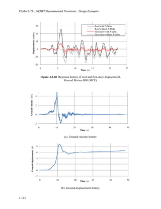
7 – 64
Table 7-18, but since the 7,000 psi concrete extends up to Level 4, not Level 8, the vertical extent of the
boundary elements is unchanged.
It is expected that the increase in concrete strength (and thus the modulus of elasticity) at the lower floors
will have a slight impact on the overall building stiffness, but this will not impact the overall design.
However, this should be verified.
Figure 7-26 Variations of neutral axis depth
(1.0 in. = 25.4 mm, 1.0 kip = 4.45 kN)
Where special boundary elements are required, transverse reinforcement must conform to ACI 318
Section 21.9.6.4(c), which refers to ACI 318 Sections 21.6.4.2 through 21.6.4.4. In addition, this section
indicates that ACI 318 Equation 21-4 need not apply and the transverse reinforcing spacing limit of
ACI 318 Section 21.6.4.3(a) can be one-third of the least dimension of the element. Similar to columns
of special moment frames, there are requirements for spacing and total area of transverse reinforcing.
The spacing is determined as follows:
One-third of least dimension = 30/3 = 10 inches
Six longitudinal bar diameters = 6(1.125) = 6.75 inches
Dimension so = 4 + (14 - hx) / 3, where so is between 4 inches and 6 inches and hx is the maximum
horizontal spacing of hoops or cross ties.
Where hoops are used, the transverse reinforcement must satisfy ACI 318 Equation 21-5:
0.09 c c
sh
yt
sb f
A
f
⎛ ⎞
′
= ⎜ ⎟
⎜ ⎟
⎝ ⎠
If #4 hoops with two crossties in each direction are used similar to the moment frame columns, Ash = 0.80
in2
and bc = 27 inches. For fc' = 7,000 psi and fyt = 60 ksi,
s = [(0.8)(60,000)]/[0.09(27.0)(7,000)] = 2.82 inches
0
1,000
2,000
3,000
4,000
5,000
6,000
7,000
0 20 40 60 80 100
F
a
c
t
o
r
e
d
a
x
i
a
l
l
o
a
d
,
P
u
(
k
i
p
s
)
Neutral axis depth (inches)
fc' = 7 ksi fc' = 5 ksi](https://image.slidesharecdn.com/femap-751-220509234918-ab6a7ec3/85/FEMA_P-751-pdf-491-320.jpg)


![Chapter 7: Reinforced Concrete
7 – 71
1. Design for Negative Moment at the Face of the Exterior Support (Grid A)
Mu = -1.3 (567) - 0.5 (259) - 1.0 (2,557) = -3,423 inch-kips
Try two #9 bars plus one #7 bar.
As = 2 (1.00) + 0.60 = 2.60 in2
Depth of compression block, a = [2.6 (60)]/[0.85 (5) 20] = 1.83 inches
Nominal strength, Mn = [2.60 (60)] [27.4 - 1.83/2] = 4,131 inch-kips
Design strength, φ Mn = 0.9 (4,131) = 3,718 inch-kips 3,423 inch-kips OK
This reinforcement also will work for negative moment at all other supports.
2. Design for Positive Moment at the Face of the Exterior Support (Grid A)
Mu = -0.8 (567) + 1.0 (2,557) = 2,114 inch-kips
Try the minimum of two #9 bars.
As = 2 (1.00) = 2.00 in2
a = 2.00 (60)/[0.85 (5) 40] = 0.71 inch
Mn = [2.00 (60)] [27.4 – 0.71/2] = 3,246 inch-kips
φ Mn = 0.9 (3,246) = 2,921 inch-kips 2,114 inch-kips OK
This reinforcement also will work for positive moment at all other supports.
The layout of flexural reinforcement layout is shown in Figure 7-32. The top short bars are cut off
5 feet-0 inch from the face of the support. The bottom bars are spliced in Spans A'-B and C-C' with a
Class B lap length of 37 inches. Unlike special moment frames, there are no requirements that the spliced
region of the bars in intermediate moment frames be confined by hoops over the length of the splice.
Note that the steel clearly satisfies the detailing requirements of ACI 318 Section 21.3.4.1.
Figure 7-32 Longitudinal reinforcement layout for Level 6 of Frame 1
(1.0 in. = 25.4 mm, 1.0 ft = 0.3048 m)
(2) #9
20'-0
2'-6
2'-4
3'-1
#4x hoops spaced from
each support: 1 at 2, 10 at 6,
balance at 10 (typical each span).
(2) #9 (2) #9
(2) #9
(2) #9 (2) #9
(1) #7
(TYP)
5'-0
(typical)
A A' B C C' D](https://image.slidesharecdn.com/femap-751-220509234918-ab6a7ec3/85/FEMA_P-751-pdf-500-320.jpg)


 = 1,150 lb/ft
W2 = [67 psf (72 ft)](153 kips / 863 kips) = 855 lb/ft
Figure 8.1-2 identifies critical regions of the diaphragm to be considered in this design. These regions
are:
§ Joint 1: Maximum transverse shear parallel to the panels at panel-to-panel joints
§ Joint 2: Maximum transverse shear parallel to the panels at the panel-to-wall joint
§ Joint 3: Maximum transverse moment and chord force
§ Joint 4: Maximum longitudinal shear perpendicular to the panels at the panel-to-wall connection
(exterior longitudinal walls) and anchorage of exterior masonry wall to the diaphragm for out-of-
plane forces
§ Joint 5: Collector element and shear for the interior longitudinal walls
A B C D E F
W1
F F
F
F
40'-0 3 at 24'-0 = 72'-0 40'-0
152'-0
W1
W2](https://image.slidesharecdn.com/femap-751-220509234918-ab6a7ec3/85/FEMA_P-751-pdf-517-320.jpg)

![FEMA P-751, NEHRP Recommended Provisions: Design Examples
8-10
§ Joint 4 – Out-of-plane forces:
The Standard has several requirements for out-of-plane forces. None are unique to precast
diaphragms and all are less than the requirements in ACI 318 for precast construction regardless of
seismic considerations. Assuming the planks are similar to beams and comply with the minimum
requirements of Standard Section 12.14 (Seismic Design Category B and greater), the required out-
of-plane horizontal force is:
0.05(D+L)plank = 0.05(67 psf + 40 psf)(24 ft / 2) = 64.2 plf
According to Standard Section 12.11.2 (Seismic Design Category B and greater), the minimum
anchorage for masonry walls is:
400(SDS)(I) = 400(0.39)1.0 = 156 plf
According to Standard Section 12.11.1 (Seismic Design Category B and greater), bearing wall
anchorage must be designed for a force computed as:
0.4(SDS)(Wwall) = 0.4(0.39)(48 psf)(8.67 ft) = 64.9 plf
Standard Section 12.11.2.1 (Seismic Design Category C and greater) requires masonry wall
anchorage to flexible diaphragms to be designed for a larger force. Due to its geometry, this
diaphragm is likely to be classified as rigid. However, the relative deformations of the wall and
diaphragm must be checked in accordance with Standard Section 12.3.1.3 to validate this assumption.
Fp = 0.85(SDS)(I)(Wwall) = 0.85(0.39)1.0[(48 psf)(8.67 ft)] = 138 plf
(Note that since this diaphragm is not flexible, this load is not used in the following calculations.)
The force requirements in ACI 318 Section 16.5 will be described later.
§ Joint 5 – Longitudinal forces:
Wall force, F = 153 kips / 8 = 19.1 kips
Wall shear along each side of wall, Vu5 = 19.1 kips [2(36 ft) / 152 ft]/2 = 4.5 kips
Collector force at wall end, Tu5 = Cu5 = 19.1 kips - 2(4.5 kips) = 10.1 kips
§ Joint 5 – Shear flow due to transverse forces:
Shear at Joint 2, Vu2 = 46 kips
Q = A d
A = (0.67 ft) (24 ft) = 16 ft2
d = 24 ft
Q = (16 ft2
) (24 ft) = 384 ft3
I = (0.67 ft) (72 ft)3
/ 12 = 20,840 ft4
Vu2Q/I = (46 kip) (384 ft3
) / 20,840 ft4
= 0.847 kip/ft maximum shear flow
Joint 5 length = 40 ft
Total transverse shear in joint 5, Vu5 = 0.847 kip/ft) (40 ft)/2 = 17 kips
ACI 318 Section 16.5 also has minimum connection force requirements for structural integrity of precast
concrete bearing wall building construction. For buildings over two stories tall, there are force](https://image.slidesharecdn.com/femap-751-220509234918-ab6a7ec3/85/FEMA_P-751-pdf-519-320.jpg)
![Chapter 8: Precast Concrete Design
8-11
requirements for horizontal and vertical members. This building has no vertical precast members.
However, ACI 318 Section 16.5.1 specifies that the strengths “... for structural integrity shall apply to all
precast concrete structures.” This is interpreted to apply to the precast elements of this masonry bearing
wall structure. The horizontal tie force requirements for a precast bearing wall structure three or more
stories in height are:
§ 1,500 pounds per foot parallel and perpendicular to the span of the floor members. The
maximum spacing of ties parallel to the span is 10 feet. The maximum spacing of ties
perpendicular to the span is the distance between supporting walls or beams.
§ 16,000 pounds parallel to the perimeter of a floor or roof located within 4 feet of the edge at all
edges.
ACI’s tie forces are far greater than the minimum tie forces given in the Standard for beam supports and
anchorage of masonry walls. They do control some of the reinforcement provided, but most of the
reinforcement is controlled by the computed connections for diaphragm action.
8.1.1.6 Diaphragm Design and Details. The phi factors used for this example are as follows:
§ Tension control (bending and ties): φ = 0.90
§ Shear: φ = 0.75
§ Compression control in tied members: φ = 0.65
The minimum tie force requirements given in ACI 318 Section 16.5 are specified as nominal values,
meaning that φ = 1.00 for those forces.
Note that although buildings assigned to Seismic Design Category C are not required to meet ACI 318
Section 21.11, some of the requirements contained therein are applied below as good practice but shown
as optional.
8.1.1.6.1 Joint 1 Design and Detailing. The design must provide sufficient reinforcement for chord
forces as well as shear friction connection forces, as follows:
§ Chord reinforcement, As1 = Tu1/φfy = (10.5 kips)/[0.9(60 ksi)] = 0.19 in2
(The collector force from
the Joint 4 calculations at 10.1 kips is not directly additive.)
§ Shear friction reinforcement, Avf1 = Vu1/φµfy = (41.4 kips)/[(0.75)(1.0)(60 ksi)] = 0.92 in2
§ Total reinforcement required = 2(0.19 in2
) + 0.92 in2
= 1.30 in2
§ ACI tie force = (1.5 kips/ft)(72 ft) = 108 kips; reinforcement = (108 kips)/(60 ksi) = 1.80 in2
Provide four #5 bars (two at each of the outside edges) plus four #4 bars (two each at the interior joint at
the ends of the plank) for a total area of reinforcement of 4(0.31 in2
) + 4(0.2 in2
) = 2.04 in2
.
Because the interior joint reinforcement acts as the collector reinforcement in the longitudinal direction
for the interior longitudinal walls, the cover and spacing of the two #4 bars in the interior joints will be
provided to meet the requirements of ACI 318 Section 21.11.7.6 (optional):](https://image.slidesharecdn.com/femap-751-220509234918-ab6a7ec3/85/FEMA_P-751-pdf-520-320.jpg)

![Chapter 8: Precast Concrete Design
8-13
Figure 8.1-4 Anchorage region of shear reinforcement for Joint 1 and
collector reinforcement for Joint 5
(1.0 in. = 25.4 mm)
8.1.1.6.2 Joint 2 Design and Detailing. The chord design is similar to the previous calculations:
§ Chord reinforcement, As2 = Tu2/φfy = (13.0 kips)/[0.9(60 ksi)] = 0.24 in2
The shear force may be reduced along Joint 2 by the shear friction resistance provided by the
supplemental chord reinforcement (2Achord - As2) and by the four #4 bars projecting from the interior
longitudinal walls across this joint. The supplemental chord bars, which are located at the end of the
walls, are conservatively excluded here. The shear force along the outer joint of the wall where the plank
is parallel to the wall is modified as follows:
( ) ( )( )( )
2
2 2 4#4 46 0.75 60ksi 1.0 4 0.2in
Mod
u u y
V V f A
φ µ ⎡ ⎤
⎡ ⎤
= − = − ×
⎣ ⎦ ⎣ ⎦
= 36.0 kips
This force must be transferred from the planks to the wall. Using the arrangement shown in Figure 8.1-5,
the required shear friction reinforcement (Avf2) is computed as:
( ) ( )
2
2
2
36.0kips
0.60in
0.75 1.0sin26.6 cos26.6
sin cos
Mod
u
vf
y f f
V
A
f
φ µ α α
= = =
°+ °
+
Use two #3 bars placed at 26.6 degrees (2-to-1 slope) across the joint at 6 feet from the ends of the plank
(two sets per plank). The angle (αf) used above provides development of the #3 bars while limiting the
grouting to the outside core of the plank. The total shear reinforcement provided is 6(0.11 in2
) = 0.66 in2
.
Note that the spacing of these connectors will have to be adjusted at the stair location.
The shear force between the other face of this wall and the diaphragm is:
Vu2-F = 46-38.3 = 7.7 kips
The shear friction resistance provided by #3 bars in the grout key between each plank (provided for the
1.5 klf requirement of ACI 318) is computed as:
φAvffyµ = (0.75)(10 bars)(0.11 in2
)(60 ksi)(1.0) = 49.5 kips
2
2
1
2
1
1
2
2 (2) #4 anchored 4'-0
into plank at ends.](https://image.slidesharecdn.com/femap-751-220509234918-ab6a7ec3/85/FEMA_P-751-pdf-522-320.jpg)

![Chapter 8: Precast Concrete Design
8-15
Figure 8.1-5 Joint 2 transverse wall joint reinforcement
(1.0 in. = 25.4 mm, 1.0 ft = 0.3048 m)
8.1.1.6.3 Design and Detailing at Joint 3. Compute the required amount of chord reinforcement at
Joint 3 as:
As3 = Tu3/φfy = (19.0 kips)/[0.9(60 ksi)] = 0.35 in2
Use two #4 bars, As = 2(0.20) = 0.40 in2
along the exterior edges (top and bottom of the plan in
Figure 8.1-2). Require cover for chord bars and spacing between bars at splices and anchorage zones per
ACI 318 Section 21.11.7.6 (optional).
§ Minimum cover = 2.5(4/8) = 1.25 in., but not less than 2.00 in.
§ Minimum spacing = 3(4/8) = 1.50 in., but not less than 1.50 in.
Figure 8.1-6 shows the chord element at the exterior edges of the diaphragm. The chord bars extend
along the length of the exterior longitudinal walls and act as collectors for these walls in the longitudinal
direction (see the Joint 4 collector reinforcement calculations and Figure 8.1-7).
#3x 2'-6
standard hook
grouted into
each key joint
(1) #5
continuous
in joint to
anchor hooks
(2) #5 in
masonry
bond beam
#3 x standard hooks
embedded in grouted
edge cell of plank. Provide
2 sets for each plank.
2
1
71
2
2
'
-
2
2
'
-
2
Vertical
reinforcement
in wall
2 cover](https://image.slidesharecdn.com/femap-751-220509234918-ab6a7ec3/85/FEMA_P-751-pdf-524-320.jpg)
![FEMA P-751, NEHRP Recommended Provisions: Design Examples
8-16
Figure 8.1-6 Joint 3 chord reinforcement at the exterior edge
(1.0 in. = 25.4 mm)
Joint 3 must also be checked for the minimum ACI tie forces. The chord reinforcement obviously
exceeds the 16 kip perimeter force requirement. To satisfy the 1.5 kips per foot requirement, a 6 kip tie is
needed at each joint between the planks, which is satisfied with a #3 bar in each joint (0.11 in2
at 60 ksi =
6.6 kips). This bar is required at all bearing walls and is shown in subsequent details.
8.1.1.6.4 Joint 4 Design and Detailing. The required shear friction reinforcement along the wall length
is computed as:
Avf4 = Vu4/φµfy = (9.0 kips)/[(0.75)(1.0)(60 ksi)] = 0.20 in2
Based upon the ACI tie requirement, provide #3 bars at each plank-to-plank joint. For eight bars total, the
area of reinforcement is 8(0.11) = 0.88 in2
, which is more than sufficient even considering the marginal
development length, which is less favorable at Joint 2. The bars are extended 2 feet into the grout key,
which is more than the development length and equal to half the width of the plank.
The required collector reinforcement is computed as:
As4 = Tu4/φfy = (10.1 kips)/[0.9(60 ksi)] = 0.19 in2
The two #4 bars, which are an extension of the transverse chord reinforcement, provide an area of
reinforcement of 0.40 in2
.
The reinforcement required by the Standard for out-of-plane force (156 plf) is far less than the ACI 318
requirement.
Figure 8.1-7 shows this joint along the wall.
Splice bars
(2) #5 bars
(chord bars)
3
3
3±
2±
3 Grouted
chord / collector
element along exterior
edge of precast plank
Contact
lap splice
Prestressed
hollow core
plank
Artificially roughened
surfaces of void as
required
4Ø spiral of 1
4 wire
with 2 pitch over each
lap splice may be required
depending on geometry
of specific voids in plank.](https://image.slidesharecdn.com/femap-751-220509234918-ab6a7ec3/85/FEMA_P-751-pdf-525-320.jpg)
![Chapter 8: Precast Concrete Design
8-17
Figure 8.1-7 Joint 4 exterior longitudinal walls to diaphragm reinforcement
and out-of-plane anchorage
(1.0 in. = 25.4 mm, 1.0 ft = 0.3048 m)
8.1.1.6.5 Joint 5 Design and Detailing. The required shear friction reinforcement along the wall length
is computed as:
Avf5 = Vu5/φµfy = (16.9 kips)/[(0.75)(1.0)(0.85)(60 ksi)] = 0.44 in2
Provide #3 bars at each plank-to-plank joint for a total of 8 bars.
The required collector reinforcement is computed as:
As5 = Tu5/φfy = (10.1 kips)/[0.9(60 ksi)] = 0.19 in2
Two #4 bars specified for the design of Joint 1 above provide an area of reinforcement of 0.40 in2
.
Figure 8.1-8 shows this joint along the wall.
2
cover
#3x 2'-6
standard hook
grouted into
each key joint
(2) #5 in
bond beam
(2) #5 bars
in joint
(chord bars)
Vertical wall
reinforcement
beyond](https://image.slidesharecdn.com/femap-751-220509234918-ab6a7ec3/85/FEMA_P-751-pdf-526-320.jpg)


![FEMA P-751, NEHRP Recommended Provisions: Design Examples
8-22
8.1.2.5.1 Minimum Reinforcement for 2.5-inch Topping. ACI 318 Section 21.11.7.1 references
ACI 318 Section 7.12, which requires a minimum As = 0.0018bd for grade 60 welded wire reinforcement.
For a 2.5-inch topping, the required As = 0.054 in2
/ft. WWR 10×10 - W4.5×W4.5 provides 0.054 in2
/ft.
The minimum spacing of wires is 10 inches and the maximum spacing is 18 inches. Note that the
ACI 318 Section 7.12 limit on spacing of five times thickness is interpreted such that the topping
thickness is not the pertinent thickness.
8.1.2.5.2 Boundary Members. Joint 3 has the maximum bending moment and is used to determine the
boundary member reinforcement of the chord along the exterior edge. The need for transverse boundary
member reinforcement is reviewed using ACI 318 Section 21.11.7.5. Calculate the compressive stress in
the chord with the ultimate moment using a linear elastic model and gross section properties of the
topping. It is conservative to ignore the precast units, but this is not necessary since the joints between
precast units are grouted. As developed previously, the chord compressive stress is:
6Mu3/td2
= 6(4,056×12)/(2.5)(72×12)2
= 157 psi
The chord compressive stress is less than 0.2f'c = 0.2(4,000) = 800 psi. Transverse reinforcement in the
boundary member is not required.
The required chord reinforcement is:
As3 = Tu3/φfy = (57.1 kips)/[0.9(60 ksi)] = 1.06 in2
8.1.2.5.3 Collectors. The design for Joint 4 collector reinforcement at the end of the exterior longitudinal
walls and for Joint 5 at the interior longitudinal walls is the same.
As4 = As5 = Ω0Tu4/φfy = (75.8 kips)/[0.9(60 ksi)] = 1.40 in2
Use two #8 bars (As = 2 × 0.79 = 1.58 in2
) along the exterior edges, along the length of the exterior
longitudinal walls and along the length of the interior longitudinal walls. Provide cover for chord and
collector bars and spacing between bars per ACI 318 Section 21.11.7.6.
§ Minimum cover = 2.5(8/8) = 2.5 in., but not less than 2.0 in.
§ Minimum spacing = 3(8/8) = 3.0 in., but not less than 1.5 in.
Figure 8.1-9 shows the diaphragm plan and section cuts of the details and Figure 8.1-10 shows the
boundary member and chord/collector reinforcement along the edge. Given the close margin on cover,
the transverse reinforcement at lap splices also is shown.](https://image.slidesharecdn.com/femap-751-220509234918-ab6a7ec3/85/FEMA_P-751-pdf-531-320.jpg)


![Chapter 8: Precast Concrete Design
8-25
Number 3 dowels are used to provide continuity of the topping slab welded wire reinforcement across the
masonry walls. The topping is to be cast into the masonry walls as shown in Figure 8.1-12 and the
spacing of the #3 bars is set to be modular with the CMU.
Figure 8.1-12 Wall-to-diaphragm reinforcement along interior longitudinal walls - Joint 5
(1.0 in. = 25.4 mm, 1.0 ft = 0.3048 m)
The required shear reinforcement along the exterior longitudinal wall (Joint 4) is:
Avf4 = Vu4/φµfy = (27.0 kips)/[(0.75)(1.0)(0.85)(60 ksi)] = 0.71 in2
The required shear reinforcement along the interior longitudinal wall (Joint 5) is:
Avf5 = Vu5/φµfy = (50.8 kips)/[(0.75)(1.0)(0.85)(60 ksi)] = 1.32 in2
Number 3 dowels spaced at 16” o.c. provide
Av = (0.11 in2
) (40 ft x 12 in/ft) / 16 in = 3.30 in2
8.1.2.5.5 Check of Out-of-Plane Forces. At Joint 4, the out-of-plane forces are checked as follows:
Fp = 0.85 SDS I Wwall = 0.85(1.0)(1.0)(60 psf)(8.67 ft) = 442 plf
With bars at 4 feet on center, Fp = 4 ft (442 plf) = 1.77 kips.
The required reinforcement, As = 1.77 kips/(0.9)(60ksi) = 0.032 in2
. Provide #3 bars at 4 feet on center,
which provides a nominal strength of 0.11×60/4 = 1.7 klf. This detail satisfies the ACI 318 Section 16.5
Cut out alternate face shells
(16 o.c. each side) and place
topping completely through
wall and between planks
(2) #5 in
masonry
bond beam
#3x4'-0 at 16 to
lap with WWF
(2) #8
collector bars
1 clear
Vertical
reinforcement
WWF 10 x 10
W4.5 x W4.5](https://image.slidesharecdn.com/femap-751-220509234918-ab6a7ec3/85/FEMA_P-751-pdf-534-320.jpg)
![FEMA P-751, NEHRP Recommended Provisions: Design Examples
8-26
required tie force of 1.5 klf. The development length was checked in the prior example. Using #3 bars at
4 feet on center will be adequate and the detail is shown in Figure 8.1-13. The detail at Joint 2 is similar.
Figure 8.1-13 Exterior longitudinal wall-to-diaphragm reinforcement and
out-of-plane anchorage - Joint 4
(1.0 in. = 25.4 mm, 1.0 ft = 0.3048 m).
8.2 THREE-STORY OFFICE BUILDING WITH INTERMEDIATE PRECAST CONCRETE
SHEAR WALLS
This example illustrates the seismic design of intermediate precast concrete shear walls. These walls can
be used up to any height in Seismic Design Categories B and C but are limited to 40 feet for Seismic
Design Categories D, E and F.
ACI 318 Section 21.4.2 requires that yielding between wall panels or between wall panels and the
foundation be restricted to steel elements. However, the Provisions are more specific in their means to
accomplish the objective of providing reliable post-elastic performance. Provisions Section 21.4.3
(ACI 318 Sec. 21.4.4) requires that connections that are designed to yield be capable of maintaining
80 percent of their design strength at the deformation induced by the design displacement. Alternatively,
they can use Type 2 mechanical splices.
Additional requirements are contained in the Provisions for intermediate precast walls with wall piers
(Provisions Sec. 14.2.2.4 [ACI 318 Sec. 21.4.5]); however, these requirements do not apply to the solid
wall panels used for this example.
2
(2) #5 in
masonry
bond beam
(2) #8
(collector bars)
WWF 10 x10
W4.5 x W4.5
Vertical wall
reinforcement
beyond
#3x STD HK
2'-6
at 4'-0 o.c.
Cut out face shells
@ 4'-0 and place
topping into wall](https://image.slidesharecdn.com/femap-751-220509234918-ab6a7ec3/85/FEMA_P-751-pdf-535-320.jpg)


(0.10 ksf) = 1,788 kips
Considering the roof to be the same weight as a floor, the total building weight is W = 3(1,788 kips) =
5,364 kips.
8.2.4.2 Base Shear. The seismic response coefficient, Cs, is computed using Standard Equation 12.8-2:
0.283
/ 4 1
DS
S
S
C
R I
= = = 0.0708
except that it need not exceed the value from Standard Equation 12.8-3 computed as:
1 0.128
( / ) 0.29(4 /1)
D
S
S
C
T R I
= = = 0.110](https://image.slidesharecdn.com/femap-751-220509234918-ab6a7ec3/85/FEMA_P-751-pdf-539-320.jpg)

![FEMA P-751, NEHRP Recommended Provisions: Design Examples
8-32
Figure 8.2-2 Forces on the longitudinal walls
(1.0 kip = 4.45 kN, 1.0 ft = 0.3048 m)
8.2.4.4.2 Transverse Direction. Design the four 15-foot-long stairwell walls for the total shear including
5 percent accidental torsion (Standard Sec. 12.8.4.2). A rough approximation is used in place of a more
rigorous analysis considering all of the walls. The maximum force on the walls is computed as follows:
V = 380/4 + 380(0.05)(150)/[(100 ft moment arm) × (2 walls in each set)] = 109 kips
Thus:
Fr = 109(0.50) = 54.5 kips
F3 = 109(0.333) = 36.3 kips
F2 = 109(0.167) = 18.2 kips
Seismic forces on the transverse walls of the stairwells are shown in Figure 8.2-3.
12'-0
12'-0
12'-0
95 kips
63.5 kips
31.5 kips
Grade
25'-0
V = ∑F = 190 kips](https://image.slidesharecdn.com/femap-751-220509234918-ab6a7ec3/85/FEMA_P-751-pdf-541-320.jpg)


![Chapter 8: Precast Concrete Design
8-35
The effective moment arm is:
jd = 25 - 1.5 = 23.5 ft
and the net tension on the uplift side is:
min 5,320 239
2 23.5 2
u
P
M
T
jd
= − = − = 107 kips
The required reinforcement is:
As = Tu/φfy = (107 kips)/[0.9(60 ksi)] = 1.98 in2
Use two #9 bars (As = 2.0 in2
) at each end with Type 2 couplers for each bar at each panel joint. Since the
flexural reinforcement must extend a minimum distance, d, (the flexural depth) beyond where it is no
longer required, use both #9 bars at each end of the panel at all three levels for simplicity. Note that if it
is desired to reduce the bar size up the wall, the design check of ACI 318 Section 21.4.3 must be applied
to the flexural strength calculation at the upper wall panel joints.
At this point a check per ACI 318 Section 16.5 will be made. Bearing walls must have vertical ties with a
nominal strength exceeding 3 kips per foot and there must be at least two ties per panel. With one tie at
each end of a 25-foot panel, the demand on the tie is:
Tu = (3 kip/ft)(25 ft)/2 = 37.5 kips
The two #9 bars are more than adequate for the ACI requirement.
Although no check for confinement of the compression boundary is required for intermediate precast
shear walls, it is shown here for interest. Using the check from ACI 318 Section 21.9.6, the depth to the
neutral axis is:
§ Total compression force, As fy + Pmax = (2.0)(60) + 397 = 517 kips
§ Compression block, a = (517 kips)/[(0.85)(5 ksi)(8 in. width)] = 15.2 in.
§ Neutral axis depth, c = a/(0.80) = 19.0 in.
The maximum depth (c) with no boundary member per ACI 318 Equation 21-8 is:
( )
600 /
u w
l
c
h
δ
≤
where the term (δu/hw) shall not be taken as less than 0.007.
Once the base joint yields, it is unlikely that there will be any flexural cracking in the wall more than a
few feet above the base. An analysis of the wall for the design lateral forces using 50 percent of the gross
moment of inertia, ignoring the effect of axial loads and applying the Cd factor of 4 to the results gives a
ratio (δu/hw) far less than 0.007. Therefore, applying the 0.007 in the equation results in a distance, c, of
71 inches, far in excess of the 19 inches required. Thus, ACI 318 would not require transverse](https://image.slidesharecdn.com/femap-751-220509234918-ab6a7ec3/85/FEMA_P-751-pdf-544-320.jpg)
![FEMA P-751, NEHRP Recommended Provisions: Design Examples
8-36
reinforcement of the boundary even if this wall were designed as a special reinforced concrete shear wall.
For those used to checking the compression stress as an index:
( ) ( )2
389 6(5,320)
8 25 12 8 25 (12)
P M
A S
σ = + = + = 694 psi
The limiting stress is 0.2f'c, which is 1,000 psi, so no transverse reinforcement is required at the ends of
the longitudinal walls.
8.2.5.1.2 Transverse Direction. The free-body diagram of the transverse walls is shown in Figure 8.2-5.
The weight of the precast concrete stairs is 100 psf and of the roof over the stairs is 70 psf.
Figure 8.2-5 Free-body diagram of the transverse walls
(1.0 kip = 4.45 kN, 1.0 ft = 0.3048 m)
The transverse wall is similar to the longitudinal wall.
At the base:
ME = (54.5 kips)(36 ft) + (36.3 kips)(24 ft) + (18.2 kips)(12 ft) = 3,052 ft-kips
∑D = (15 ft)(48 ft)(0.1 ksf) + 2(12.5 ft / 2)(10 ft / 2)(0.07 ksf)(3) + (15 ft)(8 ft / 2)[(0.1 ksf)(3) +
(0.07 ksf)]
= 72 + 13 + 18 + 4 = 107 kips
∑L = 2(12.5 ft / 2)(10 ft / 2)(0.05 ksf)(2) + (15 ft)(8 ft / 2)(0.1 ksf)(3)
= 6 + 18 = 24 kips
12'-0
12'-0
12'-0
18.2 kips
36.3 kips
54.5 kips
12'-0
13'-6
9 9
7'-0
V C
T
D
D
D
D](https://image.slidesharecdn.com/femap-751-220509234918-ab6a7ec3/85/FEMA_P-751-pdf-545-320.jpg)
 = 3.7 kips
Pmax = 1.26(107) + 0.5(24) + 0.2(4) = 148 kips
Pmin = 0.843(107) = 90.5 kips
jd = 15 - 1.5 = 13.5 ft
Tu = (Mnet/jd) - Pmin/2 = (3,052/13.5) - 90.5/2 = 181 kips
As = Tu/φfy = (181 kips)/[0.9(60 ksi)] = 3.35 in2
Use two #10 and one #9 bars (As = 3.54 in2
) at each end of each wall with a Type 2 coupler at each bar for
each panel joint. All three bars at each end of the panel will also extend up through all three levels for
simplicity. Following the same method for boundary member check as on the longitudinal walls:
§ Total compression force, As fy + Pmax = (3.54)(60) + 148 = 360 kips
§ Compression block, a = (360 kips)/[(0.85)(5 ksi)(8 in. width)] = 10.6 in.
§ Neutral axis depth, c = a/(0.80) = 13.3 in.
Even though this wall is more flexible and the lateral loads will induce more flexural cracking, the
computed deflections are still small and the minimum value of 0.007 is used for the ratio (δu/hw). This
yields a maximum value of c = 42.9 inches, thus confinement of the boundary would not be required.
The check of compression stress as an index gives:
( ) ( )2
140 6(2,930)
8 15 12 8 15 (12)
P M
A S
σ = + = + = 951 psi
Since σ 1,000 psi, no transverse reinforcement is required at the ends of the transverse walls. Note how
much closer to the criterion this transverse wall is by the compression stress check.
The overturning reinforcement and connection are shown in Figure 8.2-6.](https://image.slidesharecdn.com/femap-751-220509234918-ab6a7ec3/85/FEMA_P-751-pdf-546-320.jpg)

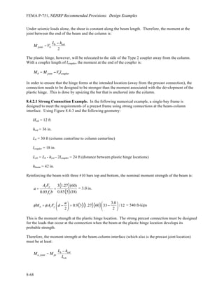

![Chapter 8: Precast Concrete Design
8-41
§ Weld at face plates, using Table 8-8 in AISC Manual (13th
edition):
φVn = φCC1Dl (2 sides)
φ =0.75
C1 = 1.0 for E70 electrodes
L = 8 in.
D = 4 (sixteenths of an inch)
K = 2 in. / 8 in. = 0.25
a = eccentricity, summed vectorally: horizontal component is 4 in.; vertical component is
2.67 in.; thus, al = 4.80 in. and a = 4.8 in. / 8 in. = 0.6 from the table. By interpolation,
C = 1.73
φVn = 0.75(1.73)(1.0)(4)(8)(2) = 83.0 kip
Weld from channel to plate has at least as much capacity, but less demand.
§ Bearing of concrete at steel channel:
fc = φ(0.85f'c) = 0.65(0.85)(5 ksi) = 2.76 ksi
The C8 has the following properties:
tw = 0.487 in.
bf = 2.53 in.
tf = 0.39 in. (average)
The bearing will be controlled by bending in the web (because of the tapered flange, the critical
flange thickness is greater than the web thickness). Conservatively ignoring the concrete’s
resistance to vertical deformation of the flange, compute the width (b) of flange loaded at 2.76 ksi
that develops the plastic moment in the web:
Mp = φFytw
2
/4 = (0.9)(50 ksi)(0.4872
in2
)/4 = 2.67 in-kip/in.
Mu = fc[(b-tw)2
/2 - (tw/2)2
/2] = 2.76[(b - 0.243 in.)2
- (0.243 in.)2
]/2
setting the two equal results in b = 1.65 inches.
Therefore, bearing on the channel is:
φVc = fc(2 - tw)(l) = (2.76 ksi)[(2(1.65) - 0.487 in.](6 in.) = 46.6 kip
To the bearing capacity on the channel is added the four #5 diagonal bars, which are effective in tension
and compression; φ = 0.75 for shear is used here:
φVs = φfyAscosα = (0.75)(60 ksi)(4)(0.31 in2
)(cos45°) = 39.5 kip
Thus, the total capacity for transfer to concrete is:
φVn = φVc + φVs = 46.6 + 39.6 = 86.1 kip](https://image.slidesharecdn.com/femap-751-220509234918-ab6a7ec3/85/FEMA_P-751-pdf-550-320.jpg)
![FEMA P-751, NEHRP Recommended Provisions: Design Examples
8-42
The capacity of the plate in the foundation is governed by the headed anchor studs. ACI 318 Appendix D
has detailed information on calculating the strength of headed anchor studs. ACI 318 Section D3.3 has
additional requirements for anchors resisting seismic forces in Seismic Design Categories C through F.
Capacity in shear for anchors located far from an edge of concrete, such as these and with sufficient
embedment to avoid the pryout failure mode is governed by the capacity of the steel, which is required by
ACI 318 Section D3.3.4:
φVsa = φ n Ase futa = (0.65)(6 studs)(0.44 in2
per stud)(60 ksi) = 103 kip
In summary, the various shear capacities of the connection are as follows:
§ Shear in the two loose angles: 130.5 kip
§ Weld at toe of loose angles: 89.1 kip
§ Weld at face plates: 83.0 kip
§ Transfer to concrete: 86.1 kip
§ Headed anchor studs at foundation: 103 kip
The number of embedded plates (n) required for a panel is:
n =402/83.0 = 4.8
Use five connection assemblies, equally spaced along each side (4'-0 on center works well to avoid the
end reinforcement). The plates are recessed to position the #5 bars within the thickness of the panel and
within the reinforcement of the panel.
It is instructive to consider how much moment capacity is added by the resistance of these connections to
vertical lift at the joint. The vertical force at the tip of the angle that will create the plastic moment in the
leg of the angle is:
T = Mp/x = Fylt2
/4 / (l-k) = (36 ksi)(8 in.)(0.31252
in2
)/4]/(4 in. - 0.69 in.) = 2.12 kips
There are five assemblies with two loose angles each, giving a total vertical force of 21 kips. The
moment resistance is this force times half the length of the panel, which yields 265 ft-kips. The total
demand moment, for which the entire system is proportioned, is 5,320 ft-kips. Thus, these connections
will add approximately 5 percent to the resistance and ignoring this contribution is reasonable. If a
straight plate measuring 1/4 inch by 8 inches (which would be sufficient) were used and if the welds and
foundation embedment did not fail first, the tensile capacity would be 72 kips each, a factor of 42 increase
over the angles and the shear connections would have the unintended effect of more than doubling the
flexural resistance, which would require a much higher shear force to develop a plastic hinge at the wall
base.
Using ACI 318 Section 11.10, check the shear strength of the precast panel at the first floor:
( ) ( )( )( )
'
2 0.75 2 5,000 8 23.5 12
c cv c
V A f hd
φ φ
= = = 239 kips](https://image.slidesharecdn.com/femap-751-220509234918-ab6a7ec3/85/FEMA_P-751-pdf-551-320.jpg)

![FEMA P-751, NEHRP Recommended Provisions: Design Examples
8-44
( )( )( ) ( )
2
0.9 ( / 2) 0.9 2.0 in 60 ksi 23.5 ft + 285 kips (23.5 ft/2)
n s y max
M A f jd P jd
φ ⎡ ⎤
⎡ ⎤
= + =
⎣ ⎦ ⎣ ⎦
= 5,552 ft-kips
Therefore, the non-yielding flexural connection at Level 2 must be strengthened.
Provide:
6,433 285
2 23.5 2
u min
u
M P
T
jd
= − = − = 131 kips
The required reinforcement is:
As = Tu/φfy = (131 kips)/[0.9(60 ksi)] = 2.43 in2
In addition to the two #9 bars that extend to the roof, provide one #6 bar developed into the wall panel
above and below the joint. Note that no increase on the development length for the #6 bar is required for
this connection since the connection itself has been designed for the loads to promote base yielding per
Provisions Section 21.4.4 (ACI 318 Sec. 21.4.3).
Since the Level 2 connection is prevented from yielding, shear friction can reasonably be used to resist
shear sliding at this location. Also, because of the lack of flexural yield at the joint, it is not necessary to
make the shear connection flexible with respect to vertical movement should an embedded plate detail be
desired.
The design shear for this location is:
Vu,Level 2 = 1.5(1.41)(95+63.5) = 335 kips
Using the same recessed embedded plate assemblies in the panel as at the base, but welded with a straight
plate, the number of plates, n, is 335/83.0 = 4.04. Use four plates, equally spaced along each side.
Figure 8.2-8 shows the shear connection at the second and third floors of the longitudinal precast concrete
shear wall panels.](https://image.slidesharecdn.com/femap-751-220509234918-ab6a7ec3/85/FEMA_P-751-pdf-553-320.jpg)


2 = 236 kips
Total building weight for seismic lateral load, W = 138+236 = 374 kips
8.3.4.2 Base Shear. The seismic response coefficient (Cs) is computed using Standard Equation 12.8-2
as:
1.0
/ 4 /
DS
S
S
C
R I I
= = = 0.25
except that it need not exceed the value from Standard Equation 12.8-3, as follows:
1 0.52
( / ) 0.189(4 /1)
D
S
S
C
T R I
= = = 0.69
where T is the fundamental period of the building computed using the approximate method of Standard
Equation 12.8-7:
( )0.75
(0.02) 20.0
x
a r n
T C h
= = = 0.189 sec
Therefore, use Cs = 0.25, which is larger than the minimum specified in Standard Equation 12.8-5:
Cs = 0.044(SDS)(I) ≥ 0.01 = 0.044(1.0)(1.0) = 0.044
The total seismic base shear is then calculated using Standard Equation 12.8-1, as:
V = CsW = (0.25)(374) = 93.5 kips
8.3.4.3 Horizontal Shear Distribution and Torsion. Torsion is not considered in the shear distribution
in buildings with flexible diaphragms. The shear along each side of the building will be equal, based on a
tributary area force distribution.](https://image.slidesharecdn.com/femap-751-220509234918-ab6a7ec3/85/FEMA_P-751-pdf-559-320.jpg)


![Chapter 8: Precast Concrete Design
8-59
( )
1.52 85,000 12
13,800
227 3,240
E
z
M
P
A S
σ
×
= + = + = 539 ksi
Roof live loads need not be included as a factored axial load in the compressive stress check, but the force
from the prestress steel will be added to the compression stress above because the prestress force will be
effective a few feet above the base and will add compression to the DT leg. Each leg of the DT will be
reinforced with one 1/2-inch-diameter strand and one 3/8-inch-diameter strand. Figure 8.3-7 shows the
location of these prestressed strands.
Figure 8.3-7 Cross section of one DT leg showing the location of
the bonded prestressing tendons or strand
(1.0 in = 25.4 mm, 1.0 ft = 0.3048 m)
Next, compute the compressive stress resulting from these strands. Note that the moment at the height of
strand development above the footing, about 26 inches for the effective stress (fse), is less than at the top
of footing. This reduces the compressive stress by:
( )
4.25 (26)
1,000
3,240
× = 34 psi
In each leg, use:
P = 0.58fpu Aps = 0.58(270 ksi)[0.153 + 0.085] = 37.3 kips
A = 168 in2
e = yb - CGStrand = 9.48 - 8.57 = 0.91 in.
Deck mesh
(1) 1
2 dia. strand
(1) 3
8 dia. strand
Leg mesh
43
4
average
2
1
2
4
6](https://image.slidesharecdn.com/femap-751-220509234918-ab6a7ec3/85/FEMA_P-751-pdf-568-320.jpg)
![FEMA P-751, NEHRP Recommended Provisions: Design Examples
8-60
Sb = 189 in3
( )
0.91 37,300
37,300
168 189
P Pe
A S
σ = + = + = 402 psi
Therefore, the total compressive stress is approximately 539 + 402 - 34 = 907 psi.
Since yielding is restricted to the steel angle and the DT is designed to be 1.5 times stronger than the yield
force in the steel angle, the full strength of the strand can be used to resist axial forces in the DT stem,
without concern for yielding in the strand.
D2 = (0.042)(20.83)(8) = 7.0 kips
Pmin = 0.7(7.0 + 2(1.08)) = 6.41 kips
ME = (1.52)(4.25)(17.83) = 115.2 ft-kips
Tu,stem = ME/d - Pmin/2= 25.5 kips
The area of tension reinforcement required is:
Aps = Tu,stem/φfpy = (25.5 kips)/[0.9(270 ksi)] = 0.10 in2
The area of one 1/2-inch-diameter strand and one 3/8-inch-diameter strand is 0.153 in2
+ 0.085 in2
=
0.236 in2
. The mesh in the legs is available for tension resistance but is not required in this check.
To determine the nominal shear strength of the concrete for the connection design, complete the shear
calculation for the panel in accordance with ACI 318 Section 11.9. The demand on each panel is:
Vu = Vpr = 6.46 kips
Only the deck between the DT legs is used to resist the in-plane shear (the legs act like flanges, meaning
that the area effective for shear is the deck between the legs). First, determine the minimum required
shear reinforcement based on ACI 318 Section 11.9.
( )( ) ( )( )
'
2 0.75 2 1.0 5,000 2.5 48
c c
V f hd
φ φ λ
= = = 12.7 kips
Since Vu of 6.46 kips exceeds φVu/2 of 6.36 kips, provide minimum reinforcement per ACI 318
Section 11.9.9.2. Using welded wire reinforcement, the required areas of reinforcement are:
Av = Avh = (0.0025)(2.5)(12) = 0.075 in2
/ft
Provide 6×6 – W4.0×W4.0 welded wire reinforcement.
Asv = Ash = 0.08 in2
/ft
The prestress force and the area of the DT legs are excluded from the calculation of the nominal shear
strength of the DT wall panel. The prestress force is not effective at the base, where the connection is and
the legs are like the flanges of a channel, which are not effective in shear.](https://image.slidesharecdn.com/femap-751-220509234918-ab6a7ec3/85/FEMA_P-751-pdf-569-320.jpg)
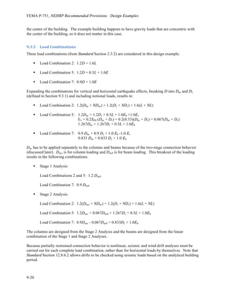
![FEMA P-751, NEHRP Recommended Provisions: Design Examples
8-62
8.3.5.6 Tension and Shear at the DT Embedment. The area of reinforcement for the welded bars of the
embedded plate in the DT, which develops tension as the angle bends through cycles, is:
( )( )
, 27.0
cos 0.9 60 cos6.3
u s e
s
y
t m
T
A
f
φ θ
= =
°
= 0.503 in2
Two #5 bars are adequate. Note that the bars in the DT leg are required to extend upward the
development length of the bar, which would be 22 inches. In this case, they will be extended 22 inches
past the point of development of the effective stress in the strand, which totals approximately 48 inches.
The same embedded plate used for tension will also be used to resist one-half the nominal shear. This
shear force is 6.46 kips. The transfer of direct shear to the concrete is easily accomplished with bearing
on the sides of the reinforcing bars welded to the plate. Two #5 and two #4 bars (explained later) are
welded to the plate. The available bearing area is approximately Abr = 4(0.5 in.)(5 in.[available]) = 10 in2
and the bearing capacity of the concrete is φVn = (0.65)(0.85)(5 ksi)(10 in2
) = 27.6 kips, which is greater
than the 6.46 kip demand.
The weld of these bars to the plate must develop both the tensile demand and this shear force. The weld
is a flare bevel weld, with an effective throat of 0.2 times the bar diameter along each side of the bar.
(Refer to the PCI Handbook.) Using the weld capacity for the #5 bar:
φVn = (0.75)(0.6)(70 ksi)(0.2)(0.625 in.)(2) = 7.9 kips/in
The shear demand is prorated among the four bars as (6.46 kip)/4 = 1.6 kips. The tension demand is
Tu,stem/2(13.5 kips). The vectorial sum of shear and tension demand is 13.6 kips. Thus, the minimum
length of weld is 13.6/7.9 = 1.7 inches.
8.3.5.7 Resolution of Eccentricities at the DT Embedment. Check the twisting of the embedded plate
in the DT for Mz. Use Mz = 24.4 in-kips.
( )
24.4
( ) 0.9 60 (9.0)
z
s
y
M
A
f jd
φ
= = = 0.05 in2
Use one #4 bar on each side of the vertical embedded plate in the DT as shown in Figure 8.3-9. This is
the same bar used to transfer direct shear in bearing.
Check the DT embedded plate for My (equal to 22.6 in-kips) and Mx (equal to 94.5 in-kips) using the two
#4 bars welded to the back side of the plate near the corners of the weld on the loose angle and the two #3
bars welded to the back side of the plate near the bottom of the DT leg (as shown in Figure 8.3-9). It is
relatively straightforward to compute the resultant moment magnitude and direction, assume a triangular
compression block in the concrete and then compute the resisting moment. It is quicker to make a
reasonable assumption as to the bars that are effective and then compute resisting moments about the X
and Y axes. That approximate method is demonstrated here. The #5 bars are effective in resisting Mx and
one each of the #3 and #5 bars are effective in resisting My. For My assume that the effective depth
extends 1 inch beyond the edge of the angle (equal to twice the thickness of the plate). Begin by
assigning one-half of the “corner” #5 bar to each component.](https://image.slidesharecdn.com/femap-751-220509234918-ab6a7ec3/85/FEMA_P-751-pdf-571-320.jpg)


![FEMA P-751, NEHRP Recommended Provisions: Design Examples
9-8
Figure 9.2-1 Typical interior W18x35 PRCC
Figure 9.2-2 Typical spandrel W21x44 PRCC
Standard double angle
shear connection
w/ A36 2L4x4x1/4
w/ 4- 3/4 dia. A325-N-SC bolts
Centerline beam
Centerline connection
OVS holes
in column
at seat angle
A36 L8x6x1/2x0'-9 (SLV)
w/4- 1 dia. A490-X-SC
bolts in horiz. leg
2- 1 dia. A490-X-SC bolts
in vert. leg
W18x35
Place transverse reinf.
below top of studs,
See 9.2-3 for number and layout
8 - #4 Long bars
see 9.2-3 for layout
One row 3/4 dia.
studs spaced @ 6
2
2
23
4
23
4
23
4
4
1
2
3 3
4
1
2
1
1
2
1
1
2
3
3
3
7
5
3
4
Standard double angle
shear connection
w/ A36 2L4x4x1/4
w/ 5-3/4 dia. A325-N-SC bolts
Centerline beam
Centerline connection
OVS holes
in column
at seat angle
A36 L8x6x5/8x0'-9 (SLV)
w/4- 1 dia. A490-X-SC
bolts in horiz. leg
2- 1 dia. A490-X-SC bolts
in vert. leg.
W21x44
Place transverse reinf.
below top of studs
See 9.2-4 for number and layout 8#5 long. bars
see 9.2-4 for layout
Drill hole in flange
for bars
One row 3/4 dia.
studs spaced @ 6
[2 rows @6 req'd @ 12.5 foot bays]
4
1
2
3 3
4
1
2
3
1
4
2
2
23
4
23
4
1
2 gap
1
1
2
1
1
2
3
3
3
1'-0
5/8 dia. x 24 long DBA
match number and spacing
of transverse reinf.
3
4
23
4](https://image.slidesharecdn.com/femap-751-220509234918-ab6a7ec3/85/FEMA_P-751-pdf-587-320.jpg)


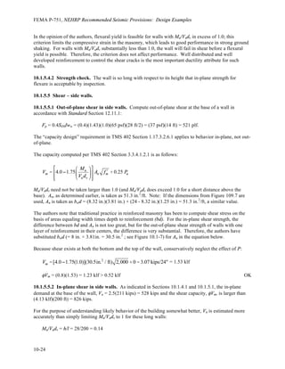


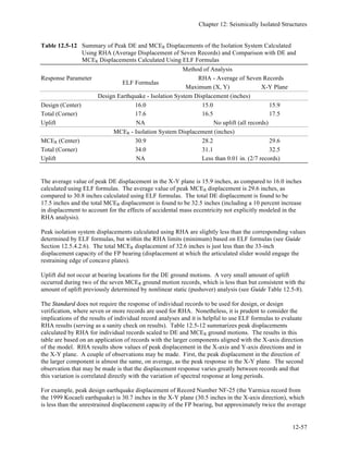


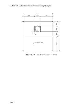


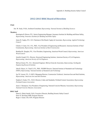


This document provides an introduction and overview of the 2009 NEHRP Recommended Seismic Provisions: Design Examples. It describes the evolution of earthquake engineering and the role of the NEHRP Provisions in establishing seismic design requirements for building codes in the United States. It also outlines the purpose and organization of the design examples, which is to illustrate the application of the NEHRP Provisions through example structural designs. The examples are intended to assist engineers who are relatively new to seismic design by demonstrating how to analyze structures and proportion structural elements according to the Provisions.


