Similar to Explainable artificial-intelligence-xai-for-exploring-spatial-variability-of-lung-and-bronchus-cancer-lbc-mortality-rates-in-the-contiguous-usa scientific-reports
Technology R&D Theme 2: From Descriptive to Predictive NetworksAlexander Pico
Similar to Explainable artificial-intelligence-xai-for-exploring-spatial-variability-of-lung-and-bronchus-cancer-lbc-mortality-rates-in-the-contiguous-usa scientific-reports (20)
1. 1
Vol.:(0123456789)
Scientific Reports | (2021) 11:24090 | https://doi.org/10.1038/s41598-021-03198-8
www.nature.com/scientificreports
Explainable artificial intelligence
(XAI) for exploring spatial
variability of lung and bronchus
cancer (LBC) mortality rates
in the contiguous USA
Zia U. Ahmed1*
, Kang Sun2
, Michael Shelly1
& Lina Mu3
Machine learning (ML) has demonstrated promise in predicting mortality; however, understanding
spatial variation in risk factor contributions to mortality rate requires explainability. We applied
explainable artificial intelligence (XAI) on a stack-ensemble machine learning model framework
to explore and visualize the spatial distribution of the contributions of known risk factors to lung
and bronchus cancer (LBC) mortality rates in the conterminous United States. We used five base-
learners—generalized linear model (GLM), random forest (RF), Gradient boosting machine (GBM),
extreme Gradient boosting machine (XGBoost), and Deep Neural Network (DNN) for developing
stack-ensemble models.Then we applied several model-agnostic approaches to interpret and
visualize the stack ensemble model’s output in global and local scales (at the county level).The
stack ensemble generally performs better than all the base learners and three spatial regression
models. A permutation-based feature importance technique ranked smoking prevalence as the most
important predictor, followed by poverty and elevation. However, the impact of these risk factors
on LBC mortality rates varies spatially.This is the first study to use ensemble machine learning with
explainable algorithms to explore and visualize the spatial heterogeneity of the relationships between
LBC mortality and risk factors in the contiguous USA.
Lung and bronchus cancer (LBC) is one of the most common causes of cancer death globally, accounting for
11.6% of all cancer deaths in
20181
. It contributes substantially to healthcare costs and the health burden
globally2
and is an insistent public health concern due to its low survival
rate3
. In the USA, the LBC mortality rate declined
by 48% from 1989 to
20163
, but it remains the top cause of cancer-related
death4
. An estimated 142,670 Ameri-
cans were expected to die from lung cancer in 2019, approximately 23 percent of all cancer deaths3
. LBC mortality
rates vary substantially between and within states in the
US3,5
. This variation has been mainly linked to variation
in smoking
prevalence6
. Yet, causes of lung cancer mortality are more
complex7
and are also linked with air
pollution8
, and socioeconomic
conditions3,9
. Some of these risk factors have not been previously included in the
modeling of predicting the LBC mortality
rate7,8,10–13
.
Several statistical methods and tools have been developed to analyze and report cancer incidence and mortal-
ity statistics in the USA, including the Poisson-gamma model, the multivariate conditional autoregressive model,
and Bayesian
inference14
. The state‐space method (SSM)15
and autoregressive quadratic time trend
model16
are
primarily used to estimate the total number of cancer deaths expected to occur in a given period. Numerous
studies have applied Geographically weighted (GW) models to explore the geographic relationship between
risk factors and the LBC mortality
rate7,8,17–19
. However, a traditional linear model may fail to capture complex
interactions and non-linear relationships between LBC mortality and risk factors. The increasing availability of
data and machine learning (ML) models present an opportunity to predict and identify the factors contributing
to the LBC mortality rate and help develop a strategy for targeting areas for the management of treatment. The
machine learning approach has been recently applied to other health problems such as arrhythmia
detection20
,
OPEN
1
Research and Education in Energy, Environment and Water (RENEW) Institute, University at Buffalo, 108 Cooke
Hall, Buffalo, NY 14260, USA. 2
Department of Civil, Structural and Environmental Engineering, University at
Buffalo, 230 Jarvis Hall, Buffalo, NY 14260, USA. 3
Department of Epidemiology and Environmental Health,
University at Buffalo, 273A Farber Hall, Buffalo, NY 14214, USA.*
email: zahmed2@buffalo.edu
2. 2
Vol:.(1234567890)
Scientific Reports | (2021) 11:24090 | https://doi.org/10.1038/s41598-021-03198-8
www.nature.com/scientificreports/
disease incidence21
, the mortality
rate22,23
, and cancer survival
prediction24
. Recently, stacked generalization
or stacking, or super learning, which introduces a meta-learner concept that combines multiple classifiers or
regression models, has been used to improve predictive accuracy25–27
. Some ML models are intrinsically capable
of explaining knowledge about domain relationships in data, known as the interpretability of the ML
models28
.
However, many ML models are "Black boxes," "meaning their internal logic and inner workings are hidden to the
user and even experts cannot fully understand the rationale behind their predictions" (Carvalho et al., 2019). The
lack of "transparency and accountability" of ML models can have some drawbacks when applied to healthcare,
criminal justice, and other regulated domains for high-stakes decision-making29
. Higher interpretable models
are easier to understand and explain the contribution of features in
predictions30
.
Although interpretability and explainability are often used interchangeably in ML, "explainable AI (XAI)"
typically refers to post hoc analyses and techniques used to understand a previously trained "black-box models"
or its
predictions31,32
. In particular, the Locally Interpretable Model-agnostic Explanations (LIME) technique
is model agnostic proposed by Ribeiro et al. (2016), which can be used to interpret nearly any kind of machine
learning models and their
predictions31
. The model-agnostic involves learning an interpretable model on the
black box model’s predictions, perturbing features, and seeing how the black box model
reacts33
or
both34
. The
LIME techniques have recently been used for explaining "black-box" predictions for a single observation or group
of observations35,36
. The "model agnostic greedy explanations of model predictions" or "break-down plot"37
can
be used as an alternative to the well-known geographical weighted
models7,8,17–19
to explore the spatial variability
of local contribution of risk factors to the prediction. However, applying the model agnostic greedy explana-
tions technique in the "black box" stack-ensemble model for explaining spatial heterogeneity in the relationship
between county-level LBC mortality rate and risk factors has not been attempted.
First, we evaluated the performance of multiple machine learning (base learners) and spatial regression mod-
els for county-level LBC mortality rates prediction using many risk factors. Then we developed stacked ensem-
ble models with these base learners to predict LBC mortality rates. Finally, we applied several model-agnostic
interpretation methods to investigate the effects of several well-known risk factors on LBC mortality rates in
the US, including permutation-based feature importance, partial dependence (PD), local-dependence (LD), and
accumulated-local (AL) profiles. We also applied "model greedy agnostic explanations of model predictions"
or "break-down plot" to explore and visualize the spatial distribution of the contributions of known risk factors
to LBC mortality rates in the conterminous US. Several risk factors were used to train all models: county-level
long-term average total cigarette smoking prevalence, poverty, health insurance, demography, biophysical fac-
tors (elevation, radon-zone, and urban–rural environment), and the satellite-derived annual average ambient
atmospheric concentrations of particulate matter with a diameter of 2.5 microns or less
(PM2.5), nitrogen dioxide
(NO2), sulfur dioxide
(SO2), and ozone.
Material and methods
Data. Lung and bronchus cancer (LBC) mortality rates by county. The county-level age-adjusted annual LBC
mortality rates from 2013 to 2017 were obtained from the National Vital Statistics System at the National Center
for Health Statistics of the Centers for Disease Control and
Prevention16,38,39
. The detailed extraction and age
adjustment methods of mortality data are described
elsewhere40
. Due to data suppression for reliability and con-
fidentiality, missing LBC mortality rate data in 348 counties in the contiguous USA counties were imputed with
missForest package41
in R. The out-of-bag (OOB) imputation error (MSE) estimate was 35 per 100,000. Finally,
we created a data-frame of 3107 counties in the conterminous US. We did not include Shannon county in South
Dakota due to a miss-match between the new and old FIPS codes, unique county identification numbers (Fig. 2).
Risk‑factors. We assembled a comprehensive set of county-level risk factors (Table S2) to develop models to
predict county-level LBC mortality rate in the contiguous USA. These data include variables relating to lifestyles,
socio-economy, demography, air pollution, and physical environments.
Cigarette smoking prevalence. Data on age-adjusted cigarette smoking prevalence by county from 2008 to
2012 was obtained from the Institute for Health Metrics and
Evaluation42
, which derived the data from the
results of the Behavioral Risk Factor Surveillance System (BRFSS) by using a logistic, hierarchical, mixed-effects
regression model with spatial and temporal
smoothing43
. The BRFSS is a state-based random digit dial (RDD)
telephone survey conducted annually in all states, the District of Columbia, and US territories. For the year 2008
to 2012 estimation, the root means squared error for male and female cigarette smoking was 1.9 for 100 sample
size43
. Data from 2013 to 2017 were obtained from County Health
Ranking44
, who also used BRFSS survey data
to estimate county averages of age-adjusted cigarette smoking (%) prevalence. Before 2016, up to seven survey
years of BRFSS data were aggregated to produce county estimates. The 2016 and 2017 data were obtained from
single-year 2014 and 2015 BRFSS survey data, respectively. The average (2008–2017) smoking prevalence by
county is shown in Fig. S1a.
Poverty rate. The data on the average (2012–2016) annual age-adjusted poverty data (% population below
poverty level) by county are shown in Fig. S1b. The data were obtained from the US Census Bureau’s Small Area
Income and Poverty Estimates (SAIPE) program (US Cenus45
. The county level observations from the American
Community Survey (ACS) and census data were used to predict the number of people in
poverty46
. The ACS is
an ongoing survey program conducted by the Census Bureau to provide vital population and housing informa-
tion across the
country47
.
3. 3
Vol.:(0123456789)
Scientific Reports | (2021) 11:24090 | https://doi.org/10.1038/s41598-021-03198-8
www.nature.com/scientificreports/
Uninsured percentage. Data on the portion of the population under age 65 without health insurance coverage
from 2013 to 2017 (Fig. S1c) was obtained from Small Area Health Insurance Estimates (SAHIE)
program45
.
The SAHIE program produces model-based health insurance coverage estimates for demographic groups within
counties and
states48
.
Demography. County-level demography data such as white, non-Hispanic population (%,), black or African
American, non-Hispanic population (%), Hispanic/Latino population (%), and population aged 65 and older
(%) were obtained from the US
Census49
. We used the 5-year means (2013–2017) of these data in our study
(Fig. S2a–d).
Air pollution. Particulate matter
(PM2.5). The county-level annual
PM2.5 data were derived from the daily
PM2.5 data set downloaded from the CDC data
portal50
. This county-level of 24-h average
PM2.5 concentrations
was generated by the US Environmental Protection Agency (EPA) using a Bayesian spatial downscaling fusion
model51
. For each county, annual
PM2.5 from 2006 to 2016 was averaged to yield long-term yearly averages,
which are mapped in Fig. S3a.
Nitrogen dioxide
(NO2). Population-weighted NO2 concentrations at 0.1°
×
0.1° resolution were estimated
using imagery from three satellite instruments, including the Global Ozone Monitoring Experiment (GOME),
Scanning Imaging Absorption Spectrometer for Atmospheric Chartography (SCIAMACHY), and GOME-2
satellite in combination with the GEOS-Chem chemical transport
model52
. We resampled all raster data at a
2.5 km × 2.5 km grid size using Empirical Bayesian Kriging. We then averaged the results within each county for
each year to yield a long-term annual average of
NO2 that was mapped from 2003 to 2012 (Fig. S3b).
Sulfur dioxide
(SO2). Gridded (1-degree spatial resolution) annual, mean
SO2 vertical column densities were
obtained from time-series, multi-source SO2 emission retrievals, and satellite SO2 measurements from the Ozone
Monitoring Instrument (OMI) on NASA’s Aura
satellite53
. We resampled all raster data at a 2.5 km × 2.5 km grid
size using Empirical Bayesian Kriging and then averaged the results within each county for the period from 2005
to 2015 (Fig. S3c).
Ozone. Annual county-level ozone data were derived from the Daily County-Level Ozone Concentrations
downloaded from the CDC’s data portal
(CDC54
, 2020). The daily data provide modeled predictions of ozone
levels from the EPA’s Downscaler model. The long-term average ozone concentration was generated from annual
ozone data from 2006 to 2016 and mapped from 2007 to 2016 (Fig. S3d).
Biophysical factors. Radon zone. County-level radon zone data were downloaded from the EPA Radon zone
interactive information
site55
. The radon zoning was done using indoor radon measurements, geology, aerial
radioactivity, soil parameters, and foundation types. There are three radon zones differentiated by their predicted
average indoor radon levels: Zone-1(> 4 pCi
L−1
), Zone-2 (2–4 pCi
L−1
), and Zone-3 (< 2 pCi
L−1
) (Fig. S4a).
Urban–rural counties. The data on the division of counties into urban or rural was drawn from the National
Center of Health Statistics (NCHS) data system’s Urban–Rural Classification Scheme for
Counties56
. All coun-
ties were classified into six classes based on the metropolitan statistical areas (MSA)57
. We then reclassified the
counties into four major classes: large central metro, large fringe metro, medium/small metro, and nonmetro
(Fig. S4b).
Coal counties. We classified the counties into two classes (yes
=
coal produced, no
=
no coal production)
according to the average coal production from 2006 to 2016 (Fig. S4c). We used data from the US Energy Infor-
mation Administration and the US Mine Safety and Health Administration’s annual survey of coal production
by US coal mining companies58
. Data includes coal production, company and mine information, operation type,
union status, labor hours, and employee numbers.
Elevation. We used elevation data from
USGS59
. Median elevation (m) for each county (Fig. S4d) was calcu-
lated.
Analytical methods. We developed stacked ensemble models from the output of five ML models to predict
and explain the county-level LBC mortality using many risk factors (Fig. 1). We applied a series of model-agnos-
tic interpretation methods to investigate the effects of several well-known risk factors on LBC mortality rates
in the US. Three spatial regression models were used to evaluate the performance of the stack-ensemble model.
Exploratory data analysis. Before developing the machine learning model, we explored spatial autocorrela-
tion and stratified spatial heterogeneity (SSH) of LBC mortality rates. Spatial autocorrelation assessment com-
prises statistics describing how a variable is autocorrelated through geographical
space60
. We used Getis-Ord
Gi statistics61
to quantify spatial autocorrelation of LBC mortality rates by estimating the z-scores and p-values
in each county. Larger statistically significant positive and negative z-scores indicate more intense clustering of
high low values, respectively. We used ArcGIS Spatial Statistics
Tools62
to estimate Getis-Ord Gi statistics for
spatial autocorrelation. We also estimated bivariate Local Moran I (LMI) statistics to explore the degree of linear
4. 4
Vol:.(1234567890)
Scientific Reports | (2021) 11:24090 | https://doi.org/10.1038/s41598-021-03198-8
www.nature.com/scientificreports/
association between LBC mortality rates and risk factors at a given location and the average of another variable
at neighboring areas (spatial lag).
Since our study area is vast, there is a possibility of high stratified spatial heterogeneity (SSH) which refers
to a partition of a study area, where variables are homogeneous within each stratum but not between
strata63
.
The q-statistic proposed by Wang et al.63
measures the degree of SSH in geographical space related to the ratio
between the variance of a variable within the strata and the pooled variance of an entire study area. The value of
the q-statistic range from 0 to 1, and it increases as the strength of the SSH increases. The calculated q-statistics
for all risk factors used the "factor_detector" function of "geodetector"
package63
in the R statistical computing
environment64
.
Training. Before training, the data set (n
=
3,107 counties) was randomly split using stratified random
sampling65
into sub-sets of training (70%), validation (15%), and test data (15%). We used seven Gi-bins or clus-
ters derived from Getis-Ord Gi* statistic of LBC mortality rates (Fig. 2a) as strata. The validation data was used
to optimize the ML model parameters during the tuning and training processes. The test data set was used as the
hold-out data to evaluate the model performance. The summary statistics and distribution of LBC mortality rate
and risk factors in the training, validation, and test data sets are similar to those in the entire data set (Fig. S5a,
b and Table S2).
Spatial regression models. The performance machine learning models were compared with three spatial
regression models: spatial error, spatial Lag, and geographically weighted OLS (GW-OLS). A brief description of
these models is given in supplementary information. For spatial regression analyses, "GWModel"66
and "spatial-
reg"67
packages in the R statistical computing environment were
used64
.
Figure 1.
Steps used in meta-ensemble machine learning regression models for LBC morality rates prediction.
GLM = generalized linear model, RF = random forest, GBM = Gradient boosting machine, XGBoost = extreme
gradient boosting machine, DNN = Deep Neural Network; GW-OLS = Geographically Weighted OLS Regression
(GW-OLS).
Figure 2.
(a) County-level 5 years (2013–2017) average annual Lung and Bronchus Cancer (LBC) Mortality
Rates, (b) The geographical clusters of counties with significant-high (hot spot—statistically significant positive
z-scores, red color) or low (cold spot—statistically significant negative z-scores, sky blue colors) values of the
Getis-Ord Gi* statistics for the LBC rate. LBC mortality rates and Getis-Ord Gi* Hot Spot maps were created in
ArcGIS Desktop version 10.6.162
.
5. 5
Vol.:(0123456789)
Scientific Reports | (2021) 11:24090 | https://doi.org/10.1038/s41598-021-03198-8
www.nature.com/scientificreports/
Machine learning base models. We trained the data with a generalized linear model (GLM), random for-
est (RF), Gradient boosting machine (GBM), extreme Gradient boosting machine (XGBoost), and Deep Neu-
ral Network (DNN) with several combinations of hyper-parameters. A brief description of all base learners is
given in Supplementary information. During training, we used a Random Grid Search (RGS) to find the opti-
mal parameter values for the base-learners to reduce over-fitting and enhance the prediction performance of the
models68
. The optimal hyperparameters were selected by conducting a grid-search using tenfold cross-validation
(Supplementary Information Table S3). We used 0.001 and 2 for "stopping tolerance" and "stopping rounds" as
early stopping parameters in the parameter tuning process. The best-performing model from each algorithm
was selected according to their performance during tenfold cross-validation with different-parameters combina-
tions. The root mean squared error (RMSE) was used as a performance matrix.
Stack‑ensemble models. Ensemble machine learning with stack-generalization uses a higher-level model
(meta–learner) to combine several lower-level models model as base-learners for better predict performance.
Unlike the "bagging" in the random forest or "boosting" in Gradient boosting approaches that can only combine
the same type of algorithm, stacked generalization can combine different algorithms to maximize the generali-
zation accuracy. It uses the following three steps: (1) set up a list of base-learners (level-0 space) and a meta-
learner (level-1 space), (2) train each of the base-learners and perform K-fold cross-validation predictions for
each base-learner, and (3) use these predicted values to train the meta-learner and make new predictions. The
base-level models often consist of different learning algorithms, and therefore stacking ensembles often combine
heterogeneous algorithms. The K-fold cross-validation outputs of all base learners were then trained with two
stacked ensemble models at the end. One ensemble contains all the sub-models of five learners (n = 147), and
the other includes just the best-performing model from each learner. The GLM regression model was used as a
meta-learner at level 1-space.
We used the "h2o"
package69
in the R statistical computing
environment64
to train, validate, and predict the
GLM, RF, GBM, XGBoost, DNN, and stack-ensemble models.
Model performance. The performance of all base-learners and stack-ensemble models were evaluated with a
hold-out-test data set. The diagnostic measures of prediction performance used here were the mean absolute
error (MAE) (1), and the root mean square error (RMSE) (2). Also, we used observe versus predicted plots to
visualize model performance and used simple linear regression between observed and predicted LBC-rates to
judge model performance.
where n is the number of counties, and y and ŷ are observed and predicted LBC rates in county i.
We also calculated bias and variance of all spatial regression and ML models by resampling the training data
set, repeating the model-building process, and deriving the average prediction error from the test data set. Bias
represents how far away an average model prediction ˆ
f (x)is far from the true f (x) , so, bias can be expressed as:
The variance represents how much a model prediction changes with different training data, i.e., variation in
prediction due to random sampling:
So total expected error of a model prediction is composed of bias and variance:
Explainable AI. The Permutation Feature Importance (PFI)
approach70
and Partial dependence plots (PDP)71
are primarily used to explain and visualize the output from simple machine learning models. Unlike traditional
statistical methods, the output of the stacked ensemble model is difficult to interpret since it combines differ-
ent ML
algorithms72
. Therefore, we created several agnostic "model explainers " to interpret the stack ensemble
model’s output at local and global scales. The "explainers" make a unified representation of a model for further
analysis37
.
Permutation‑based feature importance. We adopted the "model agnostic" Permutation Feature Importance
(PFI) approach70
, which measures the increase in the prediction error (drop-out loss or RMSE) of the model
(1)
MAE =
1
n
n
i=1
|(yi − ŷ)|
(2)
RMSE =
1
n
n
i=1
[yi − ŷ]2
(3)
Bias
ˆ
f (x)
= E
ˆ
f (x)
− f (x)
(4)
Var
ˆ
f (x)
= E
ˆ
f (x)2
− E
ˆ
f (x)
2
(5)
Err(x) = Bias
ˆ
f (x)
+ Var
ˆ
f (x)
+ σ
6. 6
Vol:.(1234567890)
Scientific Reports | (2021) 11:24090 | https://doi.org/10.1038/s41598-021-03198-8
www.nature.com/scientificreports/
after the feature values are permuted by breaking down the relationship between the feature and the true out-
come. This probabilistic method automatically considers interaction effects for importance
calculation73
.
Partial dependence (PD), local‑dependence (LD) and accumulated‑local (AL) profiles. It is not easy to inter-
pret complex machine learning algorithms by examining their coefficients. However, a partial dependence (PD)
profile can interpret a machine learning model’s output and visualize how the model’s predictions are influenced
by each predictor when all other predictors are being controlled. In these plots, the Y-axis value (
y
) is deter-
mined by the average of all possible model prediction values when the value of the objective predictor is at the
value indicated on the X-axis.
Partial dependence plots can produce inaccurate interpretations if the predictors are strongly correlated37
. As
an alternative to partial dependence profiles, a new visualization approach, accumulated local effects plots, has
been proposed, which is unbiased and does not require this unreliable extrapolation with correlated
predictors74
.
As accumulated-local (AL) profiles are related to local-dependence profiles (LD)37
, both were applied to sum-
marize the influence of an explanatory variable on the stack-ensemble model’s predictions in this study.
Model agnostic greedy explanations of model predictions (breakDown). We applied the break-down variable’s
contribution to visualize and describe how risk factors contribute to LBC mortality rates prediction locally (at
the county level). The objective of this approach is to decompose model predictions into parts that can be attrib-
uted to particular
variables75
. The Break-down Plots proposed by Biecek and
Burzykowski37
presents variable
attributions, i.e., the decomposition of the model’s prediction into contributions that can be attributed to dif-
ferent explanatory variables.
We used the DALEX
package76
in R Statistical Computing
Environment64
to create explainers for PFI, PD
-, LD- and AL-profiles, and local variables’ contribution in the best performing stack-ensemble model prediction.
Results
Exploratory data analysis. Figure 2a shows the spatial distribution of county-level, age-adjusted LBC
rates, averaged over 5 years (2013–2017). There was a total of 146,193 LBC -related deaths in the US during this
period. The South and Appalachian regions had mean LBC rates during the period 1998–2012 that were much
higher than the national average of 65 death per 100,000. The highest mean mortality rates were observed in
Union County in Florida, followed by several counties in the Appalachian region covering Kentucky, Tennessee,
and West Virginia, respectively. Counties with the lowest LBC mortality rates were observed in Summit County,
Utah.
The Getis-Ord Gi* hotspot analysis identifies statistically significant clusters of counties with a high mortality
rate (hot clusters) in the South, mainly in the Mississippi basin and the southern Appalachian region (Fig. 2b).
The cold clusters (or areas where the mortality rate was relatively low) occurred predominantly in the Midwest
and the western part of the country. There were some other small cold clusters of counties in the northeastern
coastal region.
The correlations between LBC mortality rate and risk factors are weak to moderate (Fig. S6). The correlations
were positive for LBC mortality rate and smoking (r = 0.623, p 0.001), PM2.5 (r = 0.425, p 0.001), SO2 (r = 0.293,
p 0.001) and poverty (r = 0.394, p 0.001), and negative for LBC mortality rate and percent Hispanic population
(r = − 0.364, p 0.001) and median elevation (r = − 0.443, p 0.001). The mean LBC mortality was significantly
lower in the large metro area than in other areas (Fig. S7a). For radon zones groups, mean LBC mortality rates
were lower in radon zones-1 (Fig. S7b). For the last 10 years, counties producing coal showed significantly higher
LBC mortality rates than other counties (Fig. S7c).
The bivariate global Moran’s I show a positive association between LBC mortality rates and smoking,
PM25,
SO2, and poverty activity and a negative association between the Hispanic population and median elevation
(Fig. S8). The bivariate LMI cluster of LBC mortality rates and twelve risk factors are presented in maps in
Fig. S9. The red color (High-High) in maps corresponds to significant clusters of high LBC mortality rates and
high prevalence of risk factors. The light red color (High-Low) in maps resembles clusters of high LBC mortality
rates and low prevalence of risk factors.
To see how the risk factors explained the spatial distribution LBC mortality rate in the conterminous
USA, we calculated q-statistic (strength of SSH) of 15 risk factors which were sorted in the order: Smok-
ing SO2 PM25 Elevation Ozone Poverty Hispanic population NO2 Population-65 yr Black popu-
lation White population Uninsured Radon zone Coal (yes/no) Urban–Rural (Table 1). The q-value of
smoking prevalence indicates a moderate stratified heterogeneity effect on LBC mortality rates distribution.
Fourteen out of 15 variables exhibit low SSH.
Base learners turning parameters. The optimum RF model had ntrees, max_depth, and sample_rate
of 576, 30, and 06, respectively. The best GBM had ntrees = 500, col_sample_rate = 0.5, max_depth = 20, min_
rows = 1.0. The best XGBoost model was found to have hyper-parameters of ntree = 350, max depth = 3, min_
row = 50, col sample rate = 75%. The DNN model had three hidden layers. Each layer had 100 neurons with a
Tanh, activation function, with very low L1 regularization and L2 regularization values to add stability and
reduce the risk of over-fitting. The optimum GLM model had alpha = 0 and lambda = 1.
Performance of base learners and stack ensemble model. The MAE values varied from 6.06 to 7.00
per 100,000, which is lower than the minimum value of the observed LBC rate, 10.1 per 100,000. All five base-
learners displayed only slight differences in their RMSE statistics. Among the base-learners, the RF and GBM
models performed better than all the other learners during the training stage (Table 2). They had lower MAE and
7. 7
Vol.:(0123456789)
Scientific Reports | (2021) 11:24090 | https://doi.org/10.1038/s41598-021-03198-8
www.nature.com/scientificreports/
RMSE statistics and explained more than 95% of the variability in LBC mortality rates for the training data set.
However, when the models were applied to the validation data set, they had relatively high MAE and RMSE sta-
tistics, indicating problems in generalizing their results beyond the training data set (i.e., generalization error).
The performance of three spatial regression models, five base-learners and two stack-ensemble models, was
further evaluated using a hold-out test data set (Table 2 and Fig. S9). The stack-ensemble model with all base
learners (N = 147) improved prediction over the five base models (level-0 space) and three traditional spatial
regression models. The improvement in the RMSE ranged between 2 and 32%. The
R2
for the predicted versus
the observed values for the test data set was 0.61 (Table 2). None of the base-learners successfully predicted the
lowest and highest LBC rates for the hold-out test data, and they over-estimated low-values and under-estimated
higher values (Fig. S10a–j).
When all models were rerun with ten randomly sampled trained data sets and validated with a test data set,
we found the
bias2
of RF, GBM, and the stack-estimable with all base-learners were significantly lower than
other models (Fig. S11a). However, the prediction variance of these models with different training data sets was
high (Fig. S11b). The highest
bias2
and the lowest variance were obtained with the spatial lag, GLM, and spatial
error models.
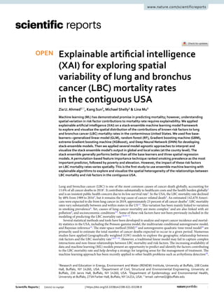
Permutation‑based variable importance. The Feature Importance (the factor by which the RMSE is
increased compared to the original model if a particular feature is permuted) of the best stack-ensemble model
is shown in Fig. 3. Among the 15 risk factors, total smoking prevalence was identified as the most important
variable, followed by poverty rate, elevation, percent white population, and
PM2.5 in the contiguous US.
Partial dependence (PD), local‑dependence (LD), and accumulated‑local (AL) profiles. Fig-
ure 4 shows partial-dependence, local-dependence, and accumulated-local profile plots of six important risk
factors. Partial dependence plots help us understand the marginal effect of a feature (or subset thereof) on the
predicted outcome. PD profiles offer a simple way to summarize a particular risk factor’s effect on the LBC
mortality rate. When other predictors were controlled for, the effects of smoking prevalence (Fig. 4a), poverty
(Fig. 4b), percentage white population (Fig. 4d), and
PM2.5 (Fig. 4f) showed a positive effect (blue lines) on
predicted LBC mortality rates. However, elevation (Fig. 4c) and percentage Hispanic population (Fig. 4e) have a
strong negative effect on expected LBC mortality rates.
Accumulated-local profiles are helpful in summarize an explanatory variable’s influence on the model’s pre-
dictions when explanatory variables are correlated. When the model is additive but, explanatory variables are
correlated, neither PD nor LD profiles will adequately capture the explanatory variable’s effect on the model’s
predictions37
. However, the AL profile will provide a correct summary of the impact of variables on prediction.
The AL and PD profiles (blue-lines Fig. 5) parallel each other for all six risk factors, suggesting that the stack-
ensemble model is additive for these six explanatory variables.
The contour plot in Fig. 5 shows the dependence of the LBC mortality rate on the joint values of two risk
factors when the effects of other risk factors are being controlled. When the average smoking prevalence is
lower than ~ 30%, LBC rates are nearly independent of poverty, whereas, for smoking prevalence rates greater
than ~ 30%, a strong dependence on poverty was observed (Fig. 5a). Similar positive interactions between smok-
ing and the percent white population (Fig. 5b) and smoking and
PM2.5 (Fig. 5d) were observed; since increases
in these risk factors are associated with an increase in the LBC mortality rate. However, smoking prevalence and
percent Hispanic population (Fig. 5c) and
PM2.5 and Elevation (Fig. 5e) interacted in opposite ways in prediction.
Table 1. Association of each feature (risk factors) with LBC mortality rates (q-values). Q-statistics measures
the strength of the stratified spatial heterogeneity (SSH).
Features q-statistic p-value
Smoking 0.3916 0.000
SO2 0.2240 0.000
PM25 0.2183 0.000
Elevation 0.2111 0.000
Ozone 0.2103 0.000
Poverty 0.1818 0.000
Hispanic population 0.1711 0.000
NO2 0.1524 0.000
Population 65 yr 0.0889 0.000
Black population 0.0494 0.000
White population 0.0483 0.000
Uninsured 0.0424 0.000
Radon zone 0.0360 0.000
Coal (yes/no) 0.0223 0.000
Urban–Rural 0.0179 0.000
8. 8
Vol:.(1234567890)
Scientific Reports | (2021) 11:24090 | https://doi.org/10.1038/s41598-021-03198-8
www.nature.com/scientificreports/
Break‑down plots for additive attributions. Break-down (BD) plots for a single observation are easy
to understand, and several risk factors’ contributions can be presented in a limited space. The BD. plots can be
used to show variable attributions, i.e., the decomposition of the model’s prediction into contributions that can
be attributed to different explanatory
variables37
. We selected two counties, Summit, Utah, and Union County,
Florida, to explore the contribution of risk factors in two contrasting environments because the lowest and high-
est LBC mortality rates were observed in these counties. The median elevation in Summit and Union Counties
are 2,587 and 47 m, respectively, and the prevalence of smoking and poverty in Summit County is lower than in
Union county. The red and green bars in Fig. 6 indicate negative and positive changes in the mean predictions
attributed to the risk factors. The most considerable negative contributions to predicting the LBC mortality
rate for Summit County, Utah, come from elevation, smoking, and poverty (Fig. 6a). The contributions of the
remaining other risk factors are smaller (in absolute values). For Union County, Florida, the predicted LBC
mortality rate is attributed to the positive contribution of smoking, poverty,
PM2.5, and radon-zone (Fig. 6b).
Figure 7 shows the spatial variability of the contribution of six risk factors for predicting LBC mortality rates
in 3107 counties. A high positive contribution of smoking was observed in many counties in the Appalachians
and the Mississippi Valley in the South and in the states of Missouri and Oklahoma (Fig. 7a). Poverty is identi-
fied as an important contributor in a large number of counties (Fig. 7b). The counties with high contributions
from poverty on the LBC mortality rate are concentrated in the Appalachians and the Mississippi Valley in the
South (Fig. 7b). Elevation, which is ranked the third most important risk factor overall, contributed negatively
in many counties in the mountain area in the West, and Appalachian regions in the South, and the North East
(Fig. 7c). In large numbers of counties in the Mid-West, North-East, and the Appalachian region in the South,
percent white pollution showed a positive contribution to the predicted LBC mortality rate (Fig. 7d). A relatively
Table 2. Mean absolute error (MAE), root mean squared error (RMSE) and the goodness of fit
(R2
) during
the training, validation, and testing stages. GLM generalized linear model, RF random forest, GBM graditent
boosting machine, XGBoost eXtreme Gradient Boosting (XGBoost), DNN deep neural networks, GW-OLS
geographically weighted OLS regression.
Models Model types Training Validation Test
MAE
Spatial lag model Spatial regression 6.57 9.24 9.02
Spatial error model Spatial regression 6.65 6.73 6.53
GW-OLS Spatial regression 5.67 6.30 6.20
GLM Base-learners 6.64 6.77 6.49
RF Base-learners 1.90 6.45 6.16
GBM Base-learners 1.21 6.54 6.20
XGBoost Base-learners 2.21 6.53 6.41
DNN Base-learners 6.01 7.47 7.00
The best of the family of the base learners Stack-ensemble 2.23 6.43 6.08
All base learners Stack-ensemble 3.95 6.39 6.06
RMSE
Spatial lag model Spatial regression 8.69 12.17 11.46
Spatial error model Spatial regression 8.82 9.12 8.35
GW-OLS Spatial regression 7.56 8.65 8.09
GLM Base-learners 8.80 9.17 8.31
RF Base-learners 2.51 8.66 8.03
GBM Base-learners 1.58 8.84 8.06
XGBoost Base-learners 3.24 8.87 8.35
DNN Base-learners 7.93 9.69 9.03
The best of the family of the base learners Stack-ensemble 3.03 8.58 7.95
All base learners Stack-ensemble 5.21 8.42 7.74
The goodness of fit (R2
)
Spatial lag model Spatial regression 0.59 0.33 0.33
Spatial error model Spatial regression 0.58 0.54 0.55
GW-OLS Spatial regression 0.69 0.59 0.58
GLM Base-learners 0.58 0.54 0.56
RF Base-learners 0.98 0.59 0.58
GBM Base-learners 0.99 0.57 0.58
XGBoost Base-learners 0.97 0.57 0.57
DNN Base-learners 0.70 0.50 0.48
The best of the family of the base learners Stack-ensemble 0.96 0.60 0.59
All base learners Stack-ensemble 0.89 0.62 0.61
9. 9
Vol.:(0123456789)
Scientific Reports | (2021) 11:24090 | https://doi.org/10.1038/s41598-021-03198-8
www.nature.com/scientificreports/
higher Hispanic population negatively contributed to LBC mortality rate prediction in several counties in Texas,
California, and New Mexico (Fig. 7e). Counties with a relatively low but positive contribution from
PM2.5 are
mostly located in the Rust Belt region in the Northeastern and Midwestern of the US and Appalachian areas
in the South (Fig. 7f).
Discussion
We demonstrated the potential use of stack-ensemble ML models and XAI to quantify and visualize the spatial
variability of several risk factors’ contributions to the LBC mortality rate across the conterminous USA. Geo-
graphically weighted (GW) models have widely been used to explore this relationship between risk factors and
the LBC mortality
rate7,8,17–19
. However, GW models have limitations in exploring the spatial relationship since
local regression coefficients are derived in locations (e.g., counties) based on the proximate area of interest and
number of
neighbors77
. To overcome this limitation, XAI with local model-agnostic interpretability and break-
down plots37
shows promise to explore risk factors’ contribution to spatial variability LBC mortality rates.
In general, interpretable MI falls into two broad categories: personalized or prediction-level interpretation
and dataset- or population-level interpretation, known as local and global interpretations,
respectively28
. The
permutation-based feature importance, a global level-interpretation, identified smoking prevalence as the most
important risk factor for LBC mortality. However, break-down plots of local model-agnostic showed a spatial
variation in smoking’s contributions to LBC mortality rate across the conterminous USA. In general, counties in
the southern states, particularly in the Appalachian region and Mississippi Valley, have high smoking prevalence
and LBC mortality
rates3,78–80
. The probability of smoking was strongly associated with compositional covariates:
poverty, education, occupation, age, sex, race/ethnicity, nativity, employment, marital status, and household
size81
. Although cigarette smoking prevalence declined from 20.9% in 2005 to 14.0% in 2017, smoking is still a
major cause of disease and death in the USA, accounting for more than 480,000 deaths every year, or about 1
in 5
deaths4
. The high LBC mortality rates in the Appalachian region and Mississippi Valley can also be partly
explained by high poverty rates, limited healthcare access, low educational attainment, and coal
mining82,83
.
We identified county-level poverty rate as the second most important risk factor for LBC mortality across the
contiguous US. Multivariate PD profile plots reveal a positive interaction between smoking and poverty rates
since increasing both features leads to increased LBC mortality rates. The relationship between socioeconomic
status and LBC mortality rates in the US is well
established13,82,84,85
. Access to health care is an economic issue,
particularly in the
US7
. The socioeconomic status, such as poverty, determines early diagnosis and treatment
and reduces the risk of death from
LBC86
. Percent population access to health insurance which is linked with
poverty contributed strongly in predicting a high LBC mortality rate in Union County, Florida, which has the
highest national LBC mortality rate.
Lung cancer incidence and mortality across the US were associated with the demographic
composition87
. In
this study, we found that the percentage of the white or Hispanic population contributed positively and nega-
tively, respectively, to the LBC mortality rate. Counties with a high proportion of white people in the Mid-West,
North-East, and the Appalachian region in the South had higher LBC mortality rates than counties in the West
Figure 3.
Permutation based feature ranking in stack-ensemble model.
10. 10
Vol:.(1234567890)
Scientific Reports | (2021) 11:24090 | https://doi.org/10.1038/s41598-021-03198-8
www.nature.com/scientificreports/
with a relatively high proportion of Hispanics. Hispanics in the US have about a 50% lower incidence rate for
lung cancer than the non-Hispanic white
population88
. Their presence contributed to lower LBC mortality rates
in the western US
generally7
. The lower LBC incidence and mortality rates in this region are probably due to
lower smoking rates in the Hispanic
population88
. We found a negative association between county-level smok-
ing prevalence and the Hispanic population (r = − 0.315, p 0.001).
After smoking and poverty, median elevation ranked third in predicting LBC mortality nationally. In many
mountainous counties in the West and North-East, elevation showed a negative contribution in prediction, which
is consistent with the conceptual model of the impact of elevation on LBC mortality
rates89
and the study of Kerry
et al.7
. Low atmospheric oxygen in higher elevation areas acts as an inhibitor of free radical damage and tumori-
genesis, which may be responsible for low incidence respiratory cancers across the US’s mountainous
counties89
.
The overall association between the LBC mortality rate and
PM2.5 and
SO2 was positive among the four air
pollutants. The shared geographic area of high LBC mortality rate, smoking, poverty, and air pollution
(PM2.5
and SO2) in the southeast and the Appalachian region indicate the association of these risk factors with higher
LBC mortality rates. Other factors, such as poor diet, genetic susceptibility, and occupational exposures, may act
independently or in concert with smoking or air pollution in determining LBC incidence and mortality90
. Inferior
air quality in these regions may synergistically contribute to a higher risk of lung cancer or respiratory
illness91,92
.
This study has some limitations. The county-level data inherent limitations since data are model-based esti-
mates from the BRFSS telephone
survey93
. Furthermore, the LBC rate data used in this study contain errors due to
the under-recording of lung cancer deaths, errors in population count, and covariates used in modeling. Besides
the limitation of the data, the post-doc explainable ML model has some
limitations29
. The XAI is usually not
suggested for high-stack discussion making due to its unreliable and unrealistic explanation of what the original
model computes. However, it is recently being used in health sectors36,94,95
. Very recently stack-ensemble model
with model agnostic methods has been applied to identify factors influencing childhood blood lead
levels72
.
Figure 4.
Partial-dependence, local-dependence, and accumulated-local profiles for the stack-ensemble model
for the (a) smoking prevalence; (b) poverty rate; (c) elevation; (d) percentage white population; (e) percentage
Hispanic population and (f) PM2.5.
11. 11
Vol.:(0123456789)
Scientific Reports | (2021) 11:24090 | https://doi.org/10.1038/s41598-021-03198-8
www.nature.com/scientificreports/
Conclusions
To our knowledge, this study is the first one to apply XAI as model greedy agnostic explanations of model predic-
tions or break-down plot37
in a stack-ensemble framework to explore the spatial variability of the contribution
of several risk factors to LBC mortality rates. Application of XAI for understanding the spatial variability of the
associations between LBC mortality rates and the risk factors may allow advanced research and policy develop-
ment to understand underlying, spatially varying contributors to LBC mortality across US counties. This study
shows strong potential for implementing XAI as a complement to or substitute for the traditional spatial regres-
sion models. This study’s findings may lead to more tailored and effective prevention strategies from a policy
perspective, which is critical, given the projected prevalence growth of LBC mortality rates in the coming decades.
Figure 5.
Two-variable partial dependence plots for the stack-ensemble modes for predicting LBC mortality
rates. (a) Smoking versus poverty; (b) smoking versus white population; (c) smoking versus Hispanic
population; (d) smoking vs. PM2.5; and (e) PM2.5 versus elevation.
Figure 6.
Break-down plots for the stack-ensemble model for the (a) Summit County, Utah, and Union County,
Florida.
12. 12
Vol:.(1234567890)
Scientific Reports | (2021) 11:24090 | https://doi.org/10.1038/s41598-021-03198-8
www.nature.com/scientificreports/
Data availability
The data sets generated during this study are available from the corresponding author upon reasonable request.
Received: 28 May 2021; Accepted: 18 November 2021
References
1. Bray, F. et al. Global cancer statistics 2018: GLOBOCAN estimates of incidence and mortality worldwide for 36 cancers in 185
countries. CA: Cancer J. Clin. 68, 394–424. https://doi.org/10.3322/caac.21492 (2018).
2. Wang, H. et al. Global, regional, and national life expectancy, all-cause mortality, and cause-specific mortality for 249 causes of
death, 1980–2015: A systematic analysis for the global burden of disease study 2015. Lancet 388, 1459–1544. https://doi.org/10.
1016/S0140-6736(16)31012-1 (2016).
3. Siegel, R. L., Miller, K. D. Jemal, A. Cancer statistics, 2019. CA: Cancer J. Clin. 69, 7–34. https://doi.org/10.3322/caac.21551
(2019).
4. Centers for Disease Control and Prevention (CDC). U.S. Cancer Statistics Working Group. https://www.cdc.gov/cancer/lung/stati
stics/ (2019).
5. Mokdad, A. H. et al. Trends and patterns of disparities in cancer mortality among US counties, 1980–2014. JAMA 317, 388–406.
https://doi.org/10.1001/jama.2016.20324 (2017).
6. Centers for Disease Control and Prevention (CDC). State-specific trends in lung cancer incidence and smoking—United States,
1999–2008. MMWR Morb. Mortal. Wkly Rep. 60, 1243 (2011).
7. Kerry, R., Goovaerts, P., Ingram, B. Tereault, C. Spatial analysis of lung cancer mortality in the American west to improve alloca-
tion of medical resources. Appl. Spat. Anal. Policy https://doi.org/10.1007/s12061-019-09331-5 (2019).
8. Moore, J. X., Akinyemiju, T. Wang, H. E. Pollution and regional variations of lung cancer mortality in the United States. Cancer
Epidemiol. 49, 118–127. https://doi.org/10.1016/j.canep.2017.05.013 (2017).
9. Albano, J. D. et al. Cancer mortality in the United States by Education level and race. JNCI: J. Natl. Cancer Inst. 99, 1384–1394.
https://doi.org/10.1093/jnci/djm127 (2007).
Figure 7.
Spatial variation of local contribution of (a) smoking, (b) poverty (c) elevation, (d) white population,
(e) Hispanic population, and (f) PM2.5 on the prediction of LBC mortality rates. The contribution of risk factors
in each county’s was calculated using break-down plots of stack-ensemble models. Maps were created in the R
(version 4.1.1) Statistical Computing
Environment64
.
13. 13
Vol.:(0123456789)
Scientific Reports | (2021) 11:24090 | https://doi.org/10.1038/s41598-021-03198-8
www.nature.com/scientificreports/
10. Winkler, V., Ng, N., Tesfaye, F. Becher, H. Predicting lung cancer deaths from smoking prevalence data. Lung Cancer 74, 170–177.
https://doi.org/10.1016/j.lungcan.2011.02.011 (2011).
11. Jeon, J. et al. Smoking and lung cancer mortality in the United States from 2015 to 2065: A comparative modeling approachsmok-
ing and lung cancer mortality in the United States From 2015 to 2065. Ann. Intern. Med. 169, 684–693. https://doi.org/10.7326/
m18-1250 (2018).
12. Singh, G. K., Siahpush, M. Williams, S. D. Changing urbanization patterns in US lung cancer mortality, 1950–2007. J. Commun.
Health 37, 412–420. https://doi.org/10.1007/s10900-011-9458-3 (2012).
13. Singh, G. K., Miller, B. A. Hankey, B. F. Changing area socioeconomic patterns in US cancer mortality, 1950–1998: Part II—Lung
and colorectal cancers. J. Natl. Cancer Inst. 94, 916–925. https://doi.org/10.1093/jnci/94.12.916 (2002).
14. Quick, H. Estimating county-level mortality rates using highly censored data from CDC WONDER. Prev. Chronic Dis. 16, 180441.
https://doi.org/10.5888/pcd16.180441external (2019).
15. Tiwari, R. C. et al. A new method of predicting US and state-level cancer mortality counts for the current calendar year. CA: Cancer
J. Clin. 54, 30–40. https://doi.org/10.3322/canjclin.54.1.30 (2004).
16. Wingo, P., Landis, S., Parker, S., Bolden, S. Heath, C. Jr. Using cancer registry and vital statistics data to estimate the number of
new cancer cases and deaths in the United States for the upcoming year. J. Reg. Manag. 25, 43–51 (1998).
17. Hu, L., Griffith, D. Chun, Y. Space-time statistical insights about geographic variation in lung cancer incidence rates: Florida,
USA, 2000–2011. Int. J. Environ. Res. Public Health 15, 2406. https://doi.org/10.3390/ijerph15112406 (2018).
18. Hu, Z. Baker, E. Geographical analysis of lung cancer mortality rate and PM2.5 using global annual average PM2.5 grids from
MODIS and MISR aerosol optical depth. J. Geosci. Environ. Prot. 5, 183–197. https://doi.org/10.4236/gep.2017.56017 (2017).
19. Hystad, P. et al. Spatiotemporal air pollution exposure assessment for a Canadian population-based lung cancer case-control study.
Environ. Health 11, 22. https://doi.org/10.1186/1476-069x-11-22 (2012).
20. Rajpurkar, P. et al. Chexnet: Radiologist-level pneumonia detection on chest x-rays with deep learning. arXiv preprint http://arxiv.
org/abs/1711.05225 (2017).
21. Christensen, T., Frandsen, A., Glazier, S., Humpherys, J. Kartchner, D. Machine Learning Methods for Disease Prediction with
Claims Data. In 2018 IEEE International Conference on Healthcare Informatics (ICHI) 467–4674. https://doi.org/10.1109/ICHI.
2018.00108 (2018).
22. Hsieh, M. H. et al. Comparison of machine learning models for the prediction of mortality of patients with unplanned extubation
in intensive care units. Sci. Rep. 8, 17116. https://doi.org/10.1038/s41598-018-35582-2 (2018).
23. Weng, S. F., Vaz, L., Qureshi, N. Kai, J. Prediction of premature all-cause mortality: A prospective general population cohort
study comparing machine-learning and standard epidemiological approaches. PLoS ONE 14, e0214365. https://doi.org/10.1371/
journal.pone.0214365 (2019).
24. Agrawal, A., Misra, S., Narayanan, R., Polepeddi, L. Choudhary, A. Lung cancer survival prediction using ensemble data mining
on seer data. Sci. Program. 20, 29–42. https://doi.org/10.1155/2012/920245 (2012).
25. Zhai, B. Chen, J. Development of a stacked ensemble model for forecasting and analyzing daily average PM2.5 concentrations
in Beijing, China. Sci. Total Environ. 635, 644–658. https://doi.org/10.1016/j.scitotenv.2018.04.040 (2018).
26. Wang, Z., Wang, K., Liu, Z., Wang, X. Pan, S. A cognitive vision method for insect pest image segmentation. IFAC-PapersOnLine
51, 85–89. https://doi.org/10.1016/j.ifacol.2018.08.066 (2018).
27. Ma, Z., Wang, P., Gao, Z., Wang, R. Khalighi, K. Ensemble of machine learning algorithms using the stacked generalization
approach to estimate the warfarin dose. PLoS ONE 13, e0205872. https://doi.org/10.1371/journal.pone.0205872 (2018).
28. Murdoch, W. J., Singh, C., Kumbier, K., Abbasi-Asl, R. Yu, B. Definitions, methods, and applications in interpretable machine
learning. Proc. Natl. Acad. Sci. 116, 22071–22080. https://doi.org/10.1073/pnas.1900654116 (2019).
29. Rudin, C. Stop explaining black box machine learning models for high stakes decisions and use interpretable models instead. Nat.
Mach. Intell. 1, 206–215. https://doi.org/10.1038/s42256-019-0048-x (2019).
30. Stiglic, G. et al. Interpretability of machine learning-based prediction models in healthcare. WIREs Data Min. Knowl. Discov. 10,
e1379. https://doi.org/10.1002/widm.1379 (2020).
31. Hall, P. Gill, N. An Introduction to Machine Learning Interpretability. O’Reilly Media (2019).
32. Gunning, D. Aha, D. DARPA’s explainable artificial intelligence (XAI) program. AI Mag. 40, 44–58. https://doi.org/10.1609/
aimag.v40i2.2850 (2019).
33. Strumbelj, E. Kononenko, I. An efficient explanation of individual classifications using game theory. J. Mach. Learn. Res. 11,
1–18. https://dl.acm.org/doi/10.5555/1756006.1756007 (2010).
34. Ribeiro, M. T., Singh, S. Guestrin, C. Model-agnostic interpretability of machine learning. arXiv preprint arxiv:1606.05386 (2016).
35. Kumarakulasinghe, N. B., Blomberg, T., Liu, J., Leao, A. S. Papapetrou, P. Evaluating Local Interpretable Model-Agnostic Expla-
nations on Clinical Machine Learning Classification Models. In 2020 IEEE 33rd International Symposium on Computer-Based
Medical Systems (CBMS) 7–12. https://doi.org/10.1109/CBMS49503.2020.00009 (2020).
36. De Sousa, I. P., Vellasco, M. M. B. R. Da Silva, E. C. Local interpretable model-agnostic explanations for classification of lymph
node metastases. Sensors 19, 2969. https://doi.org/10.3390/s19132969 (2019).
37. Biecek, P. Burzykowski, T. Explanatory Model Analysis: Explore, Explain, and Examine Predictive Models. CRC Press (2021).
38. National Center for Health Statistics (NCHS). National Vital Statistics System: Multiple Cause of Death Data File, 1980–2014 (2014).
39. Wingo, P. A. et al. Long-term trends in cancer mortality in the United States, 1930–1998. Cancer: Interdiscip. Int. J. Am. Cancer
Soc. 97, 3133–3275. https://doi.org/10.1002/cncr.11380 (2003).
40. Murphy, S., Xu, J. Kochanek, K. Deaths: Final data for 2010. National vital statistics reports. National Center for Health Statistics
61 (2013).
41. Stekhoven, D. J. Using the missForest package. R package, 1–11 (2011).
42. Institute for Health Metrics and Evaluation (IHME). United States Smoking Prevalence by County 1996–2012. Seattle, United States
of America: Institute for Health Metrics and Evaluation (IHME). http://ghdx.healthdata.org/record/ihme-data/united-states-smoki
ng-prevalence-county-1996-2012 (2014).
43. Dwyer-Lindgren, L. et al. US county-level trends in mortality rates for major causes of death, 1980–2014 US county-level trends in
mortality rates for major causes of death US county-level trends in mortality rates for major causes of death. JAMA 316, 2385–2401.
https://doi.org/10.1001/jama.2016.13645 (2016).
44. Robert Wood Johnson Foundation. Health Ranking 2020 Measures. University of Wisconsin Population Health Institute. https://
www.countyhealthrankings.org/explore-health-rankings/measures-data-sources/2020-measures (2020).
45. United States Census. Small Area Income and Poverty Estimates (SAIPE) Program. https://www.census.gov/programs-surveys/
saipe/data/datasets.html (2018).
46. Bell, W. R., Basel, W. W. Maples, J. J. An overview of the US census Bureau’s small area income and poverty estimates program.
Anal. Poverty Data Small Area Estim. 19, 379–403. https://doi.org/10.1002/9781118814963.ch19 (2016).
47. Robert Wood Johnson Foundation. The County Health Rankings. University of Wisconsin Population Health Institute. https://
www.countyhealthrankings.org/explore-health-rankings/rankings-data-documentation (2020).
48. Bowers, L., Gann, C. Upton, R. Small area health insurance estimates: 2016. Small Area Estimates. Current Population Reports
(accessed 31 July 2018); https://www.census.gov/programs-surveys/sahie.html (2018).
49. United States Census. Intercensal County Estimates by Age, Sex, Race: 1980–1989. https://www.census.gov/data/datasets/time-
series/demo/popest/1980s-county.html (2015).
14. 14
Vol:.(1234567890)
Scientific Reports | (2021) 11:24090 | https://doi.org/10.1038/s41598-021-03198-8
www.nature.com/scientificreports/
50. Centers for Disease Control and Prevention (CDC). Daily PM2.5 Concentrations All County, 2001–2016. https://data.cdc.gov/
Environmental-Health-Toxicology/Daily-PM2-5-Concentrations-All-County-2001-2016/7vdq-ztk9 (2020).
51. Berrocal, V. J., Gelfand, A. E. Holland, D. M. Space-time data fusion under error in computer model output: An application to
modeling air quality. Biometrics 68, 837–848. https://doi.org/10.1111/j.1541-0420.2011.01725.x (2012).
52. Geddes, J. A., Martin, R. V., Boys, B. L. Donkelaar, A. V. Long-term trends worldwide in ambient
NO2 concentrations inferred
from satellite observations. Environ. Health Perspect. 124, 281–289. https://doi.org/10.1289/ehp.1409567 (2016).
53. Fioletov, V. et al. Multi-source
SO2 emission retrievals and consistency of satellite and surface measurements with reported emis-
sions. Atmos. Chem. Phys. 17, 12597–12616. https://doi.org/10.5194/acp-17-12597-2017 (2017).
54. Centers for Disease Control and Prevention (CDC). Daily County-Level Ozone Concentrations, 2001–2016. https://data.cdc.gov/
Environmental-Health-Toxicology/Daily-County-Level-Ozone-Concentrations-2001-2016/kmf5-t9yc (2020).
55. U.S. Environmental Protection Agency (USEPA). EPA Map of Radon Zones Including State Radon Information and Contacts. https://
19january2017snapshot.epa.gov/radon/find-information-about-local-radon-zones-and-state-contact-information_html#radon
map (2020).
56. U.S. Department of Agriculture (USDA). Rural-Urban Continuum Codes. https://www.ers.usda.gov/data-products/rural-urban-
continuum-codes.aspx (2013).
57. Ingram, D. D. Franco, S. J. 2013 NCHS Urban-Rural Classification Scheme for Counties. Vital Health Stat. 2. 1–73 (2014).
58. U.S. Energy Information Administration (EIA). Coal Data Browser. https://www.eia.gov/coal/data/browser/ (2018).
59. U.S. Geological Survey (USGS). USGS EROS archive—Digital elevation—Shuttle radar topography mission (SRTM) void filled 1
arc-second global. Earth Resour. Obs. Sci. Cent. (2018).
60. Hardy, O. J. Vekemans, X. Isolation by distance in a continuous population: Reconciliation between spatial autocorrelation
analysis and population genetics models. Heredity 83, 145–154. https://doi.org/10.1046/j.1365-2540.1999.00558.x (1999).
61. Cliff, A. D. Ord, K. Spatial autocorrelation: A review of existing and new measures with applications. Econ. Geogr. 46, 269–
292. https://doi.org/10.2307/143144 (1970).
62. Environmental Systems Research Institute (ESRI). ArcGIS Desktop: Release 10.6.1 (2019).
63. Wang, J.-F., Zhang, T.-L. Fu, B.-J. A measure of spatial stratified heterogeneity. Ecol. Ind. 67, 250–256. https://doi.org/10.1016/j.
ecolind.2016.02.052 (2016).
64. R Core Team. R: A Language and Environment for Statistical Computing. R Foundation for Statistical Computing. https://www.R-
project.org/ (2021).
65. de Vries, P. G. Stratified Random Sampling. In: Sampling Theory for Forest Inventory (Springer, Berlin, Heidelberg). https://doi.
org/10.1007/978-3-642-71581-5_2 (1986)
66. Gollini, I., Lu, B., Charlton, M., Brunsdon, C. Harris, P. GW model: An R package for exploring spatial heterogeneity using
geographically weighted models. arXiv preprint arxiv:1306.0413 (2013).
67. Bivand, R. Piras, G. spatialreg: Spatial regression analysis. R package version, 1.1–5 (2019).
68. Hamidieh, K. A data-driven statistical model for predicting the critical temperature of a superconductor. Comput. Mater. Sci. 154,
346–354. https://doi.org/10.1016/j.commatsci.2018.07.052 (2018).
69. Aiello, S., Kraljevic, T., Maj, P. Team, C. F. T. H. O. A.
H2O: R Interface for
H2O. R Package Version, Vol. 3 (2016).
70. Fisher, A., Rudin, C. Dominici, F. Model class reliance: Variable importance measures for any machine learning model class,
from the “Rashomon” perspective. arXiv preprint arxiv:1801.01489 (2018).
71. Friedman, J. H. Greedy function approximation: A gradient boosting machine. Ann. Stat. 29, 1189–1232 (2001).
72. Liu, X., Taylor, M. P., Aelion, C. M. Dong, C. Novel application of machine learning algorithms and model-agnostic methods
to identify factors influencing childhood blood lead levels. Environ. Sci. Technol. https://doi.org/10.1021/acs.est.1c01097 (2021).
73. Molnar, C. Interpretable Machine Learning. Lulu.com (2020).
74. Apley, D. W. Zhu, J. Visualizing the effects of predictor variables in black box supervised learning models. J. Roy. Stat. Soc.: Ser.
B (Stat. Methodol.) 82, 1059–1086. https://doi.org/10.1111/rssb.12377 (2020).
75. Staniak, M. Biecek, P. Explanations of model predictions with live and breakDown packages. arXiv preprint arxiv:1804.01955
(2018).
76. Biecek, P. DALEX: Explainers for complex predictive models in R. J. Mach. Learn. Res. 19, 3245–3249. arXiv:1806.08915v2 (2018).
77. Hipp, J. A. Chalise, N. Spatial analysis and correlates of county-level diabetes prevalence, 2009–2010. Prev. Chronic Dis. 12, E08.
https://doi.org/10.5888/pcd12.140404 (2015).
78. Lengerich, E. J. et al. Cancer incidence in Kentucky, Pennsylvania, and West Virginia: Disparities in Appalachia. J. Rural Health
21, 39–47. https://doi.org/10.1111/j.1748-0361.2005.tb00060.x (2005).
79. Wingo, P. A. et al. Cancer in Appalachia, 2001–2003. Cancer 112, 181–192. https://doi.org/10.1002/cncr.23132 (2008).
80. Dwyer-Lindgren, L. et al. Cigarette smoking prevalence in US counties: 1996–2012. Popul. Health Metr. 12, 5. https://doi.org/10.
1186/1478-7954-12-5 (2014).
81. Chahine, T., Subramanian, S. V. Levy, J. I. Sociodemographic and geographic variability in smoking in the U.S.: A multilevel
analysis of the 2006–2007 current population survey, tobacco use supplement. Soc. Sci. Med. 73, 752–758. https://doi.org/10.1016/j.
socscimed.2011.06.032 (2011).
82. Mejia de Grubb, M. C. et al. Socioeconomic, Environmental, and Geographic Factors and US Lung Cancer Mortality, 1999–2009.
https://doi.org/10.15212/FMCH.2017.0108 (2017).
83. Appalachian Regional Commission and West Virginia University. Office for Social Environment and Health Research. Underlying
Socioeconomic Factors Influencing Health Disparities in the Appalachian Region: Final Report. Mary Babb Randolph Cancer
Center/Office for Social Environment and Health Research, Dept. of Community Medicine, Robert C. Byrd Health Sciences Center,
West Virginia University. http://purl.access.gpo.gov/GPO/LPS100135 (2008).
84. Boscoe, F. P. et al. The relationship between area poverty rate and site-specific cancer incidence in the United States. Cancer 120,
2191–2198. https://doi.org/10.1002/cncr.28632 (2014).
85. Boscoe, F. P., Henry, K. A., Sherman, R. L. Johnson, C. J. The relationship between cancer incidence, stage and poverty in the
United States. Int. J. Cancer 139, 607–612. https://doi.org/10.1002/ijc.30087 (2016).
86. Woods, L., Rachet, B. Coleman, M. Origins of socio-economic inequalities in cancer survival: A review. Ann. Oncol. 17,
5–19. https://doi.org/10.1093/annonc/mdj007 (2006).
87. Tabatabai, M. A. et al. Racial and gender disparities in incidence of lung and bronchus cancer in the United States: A longitudinal
analysis. PLoS ONE 11, e0162949. https://doi.org/10.1371/journal.pone.0162949 (2016).
88. Haile, R. W. et al. A review of cancer in US Hispanic populations. Cancer Prev. Res. 5, 150–163. https://doi.org/10.1158/1940-6207.
CAPR-11-0447 (2012).
89. Simeonov, K. P. Himmelstein, D. S. Lung cancer incidence decreases with elevation: Evidence for oxygen as an inhaled carcinogen.
PeerJ 3, e705. https://doi.org/10.7717/peerj.705 (2015).
90. Malhotra, J., Malvezzi, M., Negri, E., La Vecchia, C. Boffetta, P. Risk factors for lung cancer worldwide. Eur. Respir. J. 48, 889–902.
https://doi.org/10.1183/13993003.00359-2016 (2016).
91. Hamra, G. B. et al. Outdoor particulate matter exposure and lung cancer: A systematic review and meta-analysis. Environ. Health
Perspect. 122, 906–911. https://doi.org/10.1289/ehp/1408092 (2014).
92. Huang, F., Pan, B., Wu, J., Chen, E. Chen, L. Relationship between exposure to PM2.5 and lung cancer incidence and mortality:
A meta-analysis. Oncotarget 8, 43322–43331. https://doi.org/10.18632/oncotarget.17313 (2017).