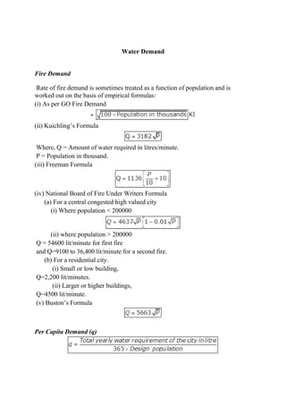
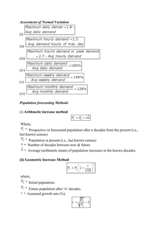
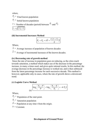
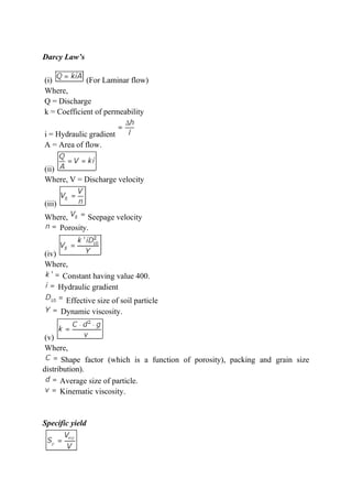
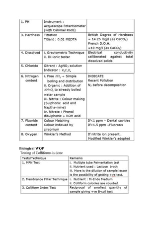
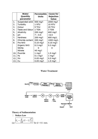
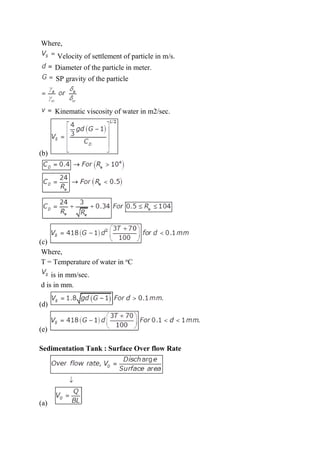
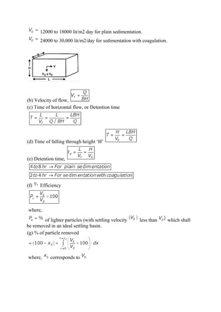
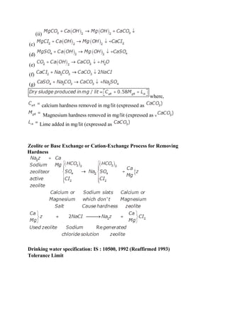
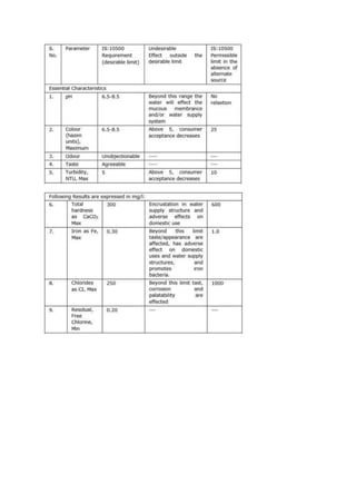
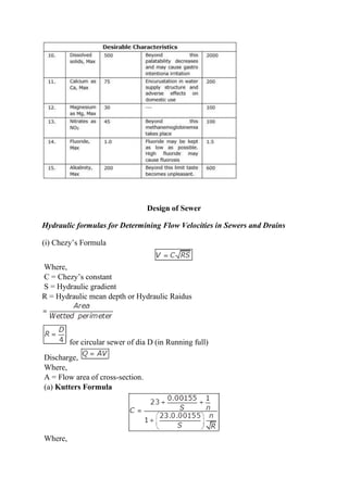
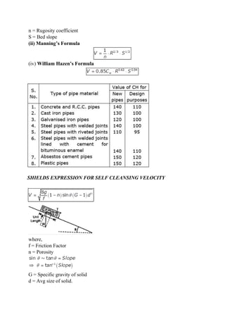
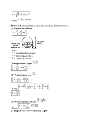
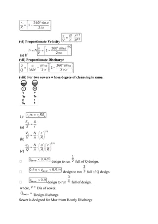
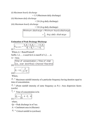
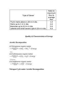
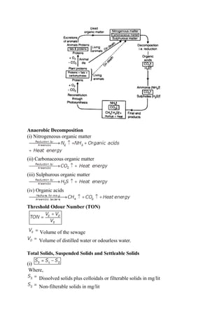
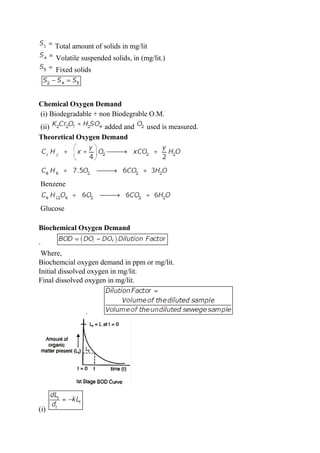
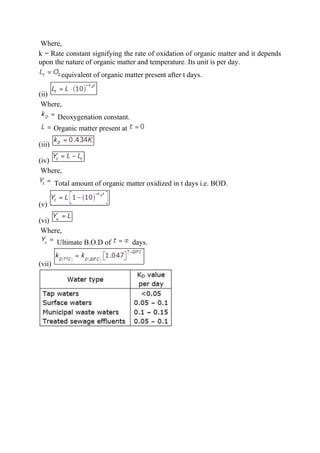
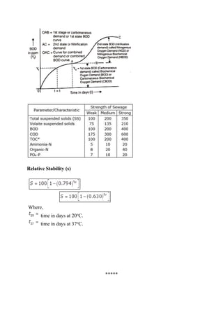
1. Water Demand
Fire Demand
Rate of fire demand is sometimes treated as a function of population and is
worked out on the basis of empirical formulas:
(i) As per GO Fire Demand
(ii) Kuichling’s Formula
Where, Q = Amount of water required in litres/minute.
P = Population in thousand.
(iii) Freeman Formula
(iv) National Board of Fire Under Writers Formula
(a) For a central congested high valued city
(i) Where population < 200000
(ii) where population > 200000
Q = 54600 lit/minute for first fire
and Q=9100 to 36,400 lit/minute for a second fire.
(b) For a residential city.
(i) Small or low building,
Q=2,200 lit/minutes.
(ii) Larger or higher buildings,
Q=4500 lit/minute.
(v) Buston’s Formula
Per Capita Demand (q)
2. Assessment of Normal Variation
(i)
(ii)
(iii)
(iv)
(v)
(vi)
Population forecasting Methods
(i) Arithmetic increase method
Where,
Prospective or forecasted population after n decades from the present (i.e.,
last known census)
Population at present (i.e., last known census)
Number of decades between now & future.
Average (arithmetic mean) of population increases in the known decades.
(ii) Geometric Increase Method
where,
Initial population.
Future population after ‘n’ decades.
Assumed growth rate (%).
3. where,
Final known population
Initial known population
Number of decades (period) between and
(iii) Incremental Increases Method
Where,
Average increase of population of known decades
Average of incremental increases of the known decades.
(iv) Decreasing rate of growth method
Since the rate of increase in population goes on reducing, as the cities reach
towards saturation, a method which makes use of the decrease in the percentage
increase, in many a times used, and gives quite rational results. In this method, the
average decrease in the percentage increase is worked out, and is then subtraced
from the latest percentage increase for each successive decade. This method is
however, applicable only in cases, where the rate of growth shows a downward
trend.
(v) Logistic Curve Method
(a)
Where,
Population of the start point.
Saturation population
Population at any time t from the origin.
Constant.
Development of Ground Water
4. Darcy Law’s
(i) (For Laminar flow)
Where,
Q = Discharge
k = Coefficient of permeability
i = Hydraulic gradient
A = Area of flow.
(ii)
Where, V = Discharge velocity
(iii)
Where, Seepage velocity
Porosity.
(iv)
Where,
Constant having value 400.
Hydraulic gradient
Effective size of soil particle
Dynamic viscosity.
(v)
Where,
Shape factor (which is a function of porosity), packing and grain size
distribution).
Average size of particle.
Kinematic viscosity.
Specific yield
5. Where, Specific yield.
Volume of water yielded under gravity effect.
Total volume of water drained.
Specific retention
Where, Specific retention.
Volume of water retain under gravity effect.
Total volume of water.
Where, Porosity.
Slot Opening
Slot size of D10 of gravel pack material.
Slot size of aquifer design on the basis of finest aquifer.
Well Losses
Jacob-equilibrium formula for confined aquifer,
Where,
Drawdown in observation well after time t.
Radial distance of observation well from main pump well.
Coefficient of transmissibility = k.d
Coefficient of storage.
Drawdown of observation well at time
Where, and is the distance of drawdown in
time and respectively.
Quality control of Water Supplies
6. Total Solid and Suspended Solid
Acceptable limit of total solid = 500 mg/lit
Threshold odour number
where, TON = Threshold odour number
constituents of Alkalinity
Major sources
Minor sources
(a)
Equivalent weight of
(b)
(c)
where,
7. Value of water
for strong acid.
for strong base
for neutral solution
Hardness of water
where,
(a)
Where,
atomic weight of Ca = 40
atomic weight of Mg = 24
atomic weight of O = 16
atomic weight C = 12
8. valency of Ca = 2
Valency of Mg = 2
(b)
(c)
Note: -ve value is taken as zero.
Biochemical Oxygen Demand (BOD)
where, of 5 days
Loss of oxygen in mg/lit.
Initial dissolved oxygen concentration in the diluted sample.
Final dissolved oxygen concentration in the diluted sample.
(After 5 day of incubation of 20o
C)
12. Where,
Velocity of settlement of particle in m/s.
Diameter of the particle in meter.
SP gravity of the particle
Kinematic viscosity of water in m2/sec.
(b)
(c)
Where,
T = Temperature of water in o
C
is in mm/sec.
d is in mm.
(d)
(e)
Sedimentation Tank : Surface Over flow Rate
(a)
13. 12000 to 18000 lit/m2 day for plain sedimentation.
24000 to 30,000 lit/m2/day for sedimentation with coagulation.
(b) Velocity of flow,
(c) Time of horizontal flow, or Detention time
(d) Time of falling through height ‘H’
(e) Detention time,
(f) Efficiency
where,
of lighter particles (with settling velocity less than which shall
be removed in an ideal settling basin.
(g) % of particle removed
where, corresponds to
14. (h) Detention time ‘t’
for rectangular tank.
for circular tank
where,
d = Dia of the tank
H = Vertical depth of wall or side water depth
(i)
(j) Scour velocity,
Where,
0.04 for unigranular sand and 0.06 or more for non-uniform (interlocking)
sticky material.
Darcy weisback friction factor.
= 0.025 to0.03 for settling tanks.
Chemicals used for Coagulation
Alum
666 gm of Alum racts with 48 gm of to give 146 gm of
15. 1 gm of Alum reacts with 0.73 gm of alk. or 0.45 gm
of alk.
to give 0.234 gm of ppt.
Filtration
A. Slow Sand Filter
Depth of filter is 2.5 to 3.5 m.
Plan area of filter is 100 to 200 m2
.
Design period = 10 years.
Depth of sand is 90 to 110 cm.
Frequency of cleaning is 1 to 3 months
Rate of filtration = 2400 to 4800 lit/m2
/day or 100 to 200 lit/m2
/hr.
Efficiency of bacteria removal = 98 to 99%.
It can not be used if turbidity > 50 ppm.
It is designed for maximum daily demand.
B. Rapid Sand Filter
where,
N = Number of unit required
Q = Plant capacity in million lit/day (MLD)
Sand layer depth is 60 to 90 cm.
16. of sand is 0.35 to 0.55 mm.
Depth of tank = 2.5 m to 3.5 m.
Area = 10 to 80 m2
each unit.
Rate of filtration 3000 to 6000 lit/m2
/hour (slow sand filter × 30)
Cross-sectional area of manford = 2 × cross-sectional area of lateral.
Cross-sectional area of each lateral = 2 to 4 times cross-sectional area of
perforations in it.
Total cross-sectional area of perforation = 0.2% of total area of 1 filter bed
4.5% of filtered water is used as back wash.
30 min. used for back wash.
Disinfection or Sterilization
(i) Treatment with Ozone
(ii) Disinfecting Action of Chlorine
17. (iii) Doses of Chlorine
(iv) Forms in which chlorine is applied
(a) Free chlorine
(b) Hypochlorites & Bleaching Powder
(c) Chloramines
(d) Chlorine dioxide
Type of Chlorination
(i) Plain chlorination
(ii) Pre-chlorination
(iii) Post-chlorination
(iv) Double chlorination
(v) Break point chlorination
(vi) Super chlorination
(vii) Dechlorination
18. Test of Chlorine Residual
1. Orthotoulidine test : colour – matching method
2. Arsenide orthotoulidine test – when mineral present in water sample, Also a
colour matching method.
3. DPD and chlorotex test (Di-ethyl phenyline diamine): colourmaking method.
4. Starch iodide Test
Water Softening
Methods of Removing Temporary hardness
(i) Boiling
(ii) Addition of lime
Method of Removing Permanent Hardness
(i) Lime-Soda Process
(a)
(b) (i)
19. (ii)
(c)
(d)
(e)
(f)
(g)
where,
calcium hardness removed in mg/lit (expressed as
Magnesium hardness removed in mg/lit (expressed as v
Lime added in mg/lit (expressed as
Zeolite or Base Exchange or Cation-Exchange Process for Removing
Hardness
Drinking water specification: IS : 10500, 1992 (Reaffirmed 1993)
Tolerance Limit
20.
21. Design of Sewer
Hydraulic formulas for Determining Flow Velocities in Sewers and Drains
(i) Chezy’s Formula
Where,
C = Chezy’s constant
S = Hydraulic gradient
R = Hydraulic mean depth or Hydraulic Raidus
for circular sewer of dia D (in Running full)
Discharge,
Where,
A = Flow area of cross-section.
(a) Kutters Formula
Where,
22. n = Rugosity coefficient
S = Bed slope
(ii) Manning’s Formula
(iv) William Hazen’s Formula
SHIELDS EXPRESSION FOR SELF CLEANSING VELOCITY
where,
f = Friction Factor
n = Porosity
G = Specific gravity of solid
d = Avg size of solid.
23. where,
Hydraulic Characteristics of Circular Sewer Free Board Provision
(i) Depth of partial flow
where,
Central angle in degree
Depth of partial flow
Dia of full section
(ii) Proportionate depth,
(iii) Proportionate area
Where,
(iv) Proportionate perimeter
Where,
(v) Proportionate Hydraulic Mean Depth
24. (vi) Proportionate Velocity
(a) If
(vii) Proportionate Discharge
(viii) For two sewers whose degree of cleansing is same.
i.e.
(a)
(b)
(c)
design to run full of Q design.
design to run full of design.
where, Dia of sewer.
Design discharge.
Sewer is designed for Maximum Hourly Discharge
25. (i) Maximum hourly discharge
= 1.5 (Maximum daily discharge)
(ii) Maximum daily discharge
= 2.0 (Avg daily discharge)
(iii) Maximum hourly discharge
= 3.0 (Avg daily discharge)
Estimation of Peak Drainage Discharge
(i)
Where, k = Runoff/rainoff
Suffix 1,2, … n used for k is runoff of 1,2, ….n.
A = Area.
(ii)
(iii)
Where,
Maximum rainfall intensity of a particular frequency having duration equal to
time of concentration.
(Point rainfall intensity of same frequency as PC) × Area dispersion factor.
(cm/hr)
Time of concentration in hr.
(iv)
where,
QP = Peak discharge in m3
/sec.
A = Catchment area in (Hectare)
Critical rainfall in (cm/hour)
26. Quality & Characteristics of Sewage
Aerobic Decomposition
(i) Nitrogenous organic matter
Nitrate
(ii) Carbonaceous organic matter
Carbondioxide
(iii) Sulphurous organic matter
Nitrogen Cycle under Aerobic Decomposition
27. Anaerobic Decomposition
(i) Nitrogeneous organic matter
(ii) Carbonaceous organic matter
(iii) Sulphurous organic matter
(iv) Organic acids
Threshold Odour Number (TON)
Volume of the sewage
Volume of distilled water or odourless water.
Total Solids, Suspended Solids and Settleable Solids
(i)
Where,
Dissolved solids plus colloidals or filterable solids in mg/lit
Non-filterable solids in mg/lit
28. Total amount of solids in mg/lit
Volatile suspended solids, in (mg/lit.)
Fixed solids
Chemical Oxygen Demand
(i) Biodegradable + non Biodegrable O.M.
(ii) added and used is measured.
Theoretical Oxygen Demand
Benzene
Glucose
Biochemical Oxygen Demand
·
Where,
Biochemcial oxygen demand in ppm or mg/lit.
Initial dissolved oxygen in mg/lit.
Final dissolved oxygen in mg/lit.
·
(i)
29. Where,
k = Rate constant signifying the rate of oxidation of organic matter and it depends
upon the nature of organic matter and temperature. Its unit is per day.
equivalent of organic matter present after t days.
(ii)
Where,
Deoxygenation constant.
Organic matter present at
(iii)
(iv)
Where,
Total amount of organic matter oxidized in t days i.e. BOD.
(v)
(vi)
Where,
Ultimate B.O.D of days.
(vii)