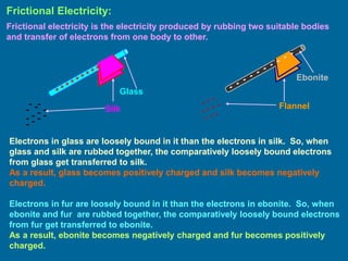
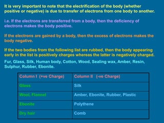
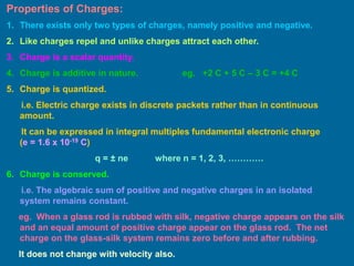
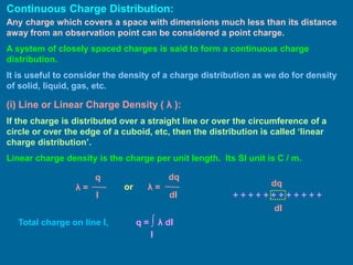
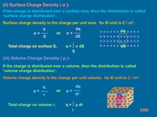
Coefficient of Thermal Expansion and their Importance.pptx
Electrostatics_1.ppt
1. ELECTROSTATICS - I
– Electrostatic Force
1. Frictional Electricity
2. Properties of Electric Charges
3. Coulomb’s Law
4. Coulomb’s Law in Vector Form
5. Units of Charge
6. Relative Permittivity or Dielectric Constant
7. Continuous Charge Distribution
i) Linear Charge Density
ii) Surface Charge Density
iii) Volume Charge Density
2. Frictional Electricity:
Frictional electricity is the electricity produced by rubbing two suitable bodies
and transfer of electrons from one body to other.
.
Glass
Silk
Ebonite
Flannel
Electrons in glass are loosely bound in it than the electrons in silk. So, when
glass and silk are rubbed together, the comparatively loosely bound electrons
from glass get transferred to silk.
As a result, glass becomes positively charged and silk becomes negatively
charged.
Electrons in fur are loosely bound in it than the electrons in ebonite. So, when
ebonite and fur are rubbed together, the comparatively loosely bound electrons
from fur get transferred to ebonite.
As a result, ebonite becomes negatively charged and fur becomes positively
charged.
3. It is very important to note that the electrification of the body (whether
positive or negative) is due to transfer of electrons from one body to another.
i.e. If the electrons are transferred from a body, then the deficiency of
electrons makes the body positive.
If the electrons are gained by a body, then the excess of electrons makes the
body negative.
If the two bodies from the following list are rubbed, then the body appearing
early in the list is positively charges whereas the latter is negatively charged.
Fur, Glass, Silk, Human body, Cotton, Wood, Sealing wax, Amber, Resin,
Sulphur, Rubber, Ebonite.
Column I (+ve Charge) Column II (-ve Charge)
Glass Silk
Wool, Flannel Amber, Ebonite, Rubber, Plastic
Ebonite Polythene
Dry hair Comb
4. Properties of Charges:
1. There exists only two types of charges, namely positive and negative.
2. Like charges repel and unlike charges attract each other.
3. Charge is a scalar quantity.
4. Charge is additive in nature. eg. +2 C + 5 C – 3 C = +4 C
5. Charge is quantized.
i.e. Electric charge exists in discrete packets rather than in continuous
amount.
It can be expressed in integral multiples fundamental electronic charge
(e = 1.6 x 10⁻¹⁹ C)
q = ± ne where n = 1, 2, 3, …………
6. Charge is conserved.
i.e. The algebraic sum of positive and negative charges in an isolated
system remains constant.
eg. When a glass rod is rubbed with silk, negative charge appears on the silk
and an equal amount of positive charge appear on the glass rod. The net
charge on the glass-silk system remains zero before and after rubbing.
It does not change with velocity also.
5. Note: Recently, the existence of quarks of charge ⅓ e and ⅔ e has been
postulated. If the quarks are detected in any experiment with concrete
practical evidence, then the minimum value of ‘quantum of charge’ will be
either ⅓ e or ⅔ e. However, the law of quantization will hold good.
Coulomb’s Law – Force between two point electric charges:
The electrostatic force of interaction (attraction or repulsion) between two point
electric charges is directly proportional to the product of the charges, inversely
proportional to the square of the distance between them and acts along the line
joining the two charges.
Strictly speaking, Coulomb’s law applies to stationary point charges.
r
q1 q2
F α q1 q2
F α 1 / r2
or F α
q1 q2
r2
F = k
q1 q2
r2
or
where k is a positive constant of
proportionality called
electrostatic force constant or
Coulomb constant.
In vacuum, k =
1
4πε0
where ε0 is the permittivity of free space
6. In medium, k =
1
4πε
where ε is the absolute electric permittivity of
the dielectric medium
The dielectric constant or relative permittivity or specific inductive capacity or
dielectric coefficient is given by
F =
q1 q2
r2
1
4πε0
In vacuum,
F =
q1 q2
r2
1
4πε0εr
In medium,
ε0 = 8.8542 x 10⁻¹² C2 N-1 m-2
= 8.9875 x 10⁹ N m2 C-2
1
4πε0
or = 9 x 10⁹ N m2 C-2
1
4πε0
K = εr =
ε
ε0
7. Coulomb’s Law in Vector Form:
r
+ q1 + q2
F21
F12
r12
q1q2 > 0
q1q2 < 0
r
+ q1 - q2
F21
F12
r12
In vacuum, for q1 q2 > 0,
q1 q2
r2
1
4πε0
r21
F12 =
q1 q2
r2
1
4πε0
r12
F21 =
In vacuum, for q1 q2 < 0,
q1 q2
r2
1
4πε0
r12
F12 =
q1 q2
r2
1
4πε0
r21
F21 =
&
F12 = - F21 (in all the cases)
r
- q1 - q2
F21
F12
r12
q1q2 > 0
8. q1 q2
r3
1
4πε0
r12
F12 =
q1 q2
r3
1
4πε0
r21
F21 =
&
Note: The cube term of the distance is simply because of vector form.
Otherwise the law is ‘Inverse Square Law’ only.
Units of Charge:
In SI system, the unit of charge is coulomb (C).
One coulomb of charge is that charge which when placed at rest in vacuum at a
distance of one metre from an equal and similar stationary charge repels it and
is repelled by it with a force of 9 x 10⁹ newton.
In cgs electrostatic system, the unit of charge is ‘statcoulomb’ or ‘esu of charge’.
In cgs electrostatic system, k = 1 / K where K is ‘dielectric constant’.
For vacuum, K = 1.
F =
q1 q2
r2
If q1 = q2 = q (say), r = 1 cm and F = 1 dyne, then q = ± 1 statcoulomb.
In cgs electromagnetic system, the unit of charge is ‘abcoulomb’ or ‘emu of
charge’.
9. 1 emu of charge = c esu of charge
1 emu of charge = 3 x 10¹⁰ esu of charge
1 coulomb of charge = 3 x 10⁹ statcoulomb
1 abcoulomb = 10 coulomb
Relative Permittivity or Dielectric Constant or Specific Inductive
Capacity or Dielectric Coefficient:
The dielectric constant or relative permittivity or specific inductive capacity or
dielectric coefficient is given by the ratio of the absolute permittivity of the
medium to the permittivity of free space.
K = εr =
ε
ε0
The dielectric constant or relative permittivity or specific inductive capacity or
dielectric coefficient can also be defined as the ratio of the electrostatic force
between two charges separated by a certain distance in vacuum to the
electrostatic force between the same two charges separated by the same
distance in that medium.
K = εr =
Fv
Fm
Dielectric constant has no unit.
10. Continuous Charge Distribution:
Any charge which covers a space with dimensions much less than its distance
away from an observation point can be considered a point charge.
A system of closely spaced charges is said to form a continuous charge
distribution.
It is useful to consider the density of a charge distribution as we do for density
of solid, liquid, gas, etc.
(i) Line or Linear Charge Density ( λ ):
If the charge is distributed over a straight line or over the circumference of a
circle or over the edge of a cuboid, etc, then the distribution is called ‘linear
charge distribution’.
Linear charge density is the charge per unit length. Its SI unit is C / m.
q
λ =
l
λ =
dq
dl
or
+ + + + + + + + + + + +
dq
dl
Total charge on line l, q = ∫ λ dl
l
11. (ii) Surface Charge Density ( σ ):
σ =
q
S
σ =
dq
dS
or
If the charge is distributed over a surface area, then the distribution is called
‘surface charge distribution’.
Surface charge density is the charge per unit area. Its SI unit is C / m2.
+ + + + + + + + + + + +
+ + + + + + + + + + + +
+ + + + + + + + + + + +
+ + + + + + + + + + + +
dq
dS
Total charge on surface S, q = ∫ σ dS
S
(iii) Volume Charge Density ( ρ ):
ρ =
q
ז
ρ =
dq
dז
or
If the charge is distributed over a volume, then the distribution is called
‘volume charge distribution’.
Volume charge density is the charge per unit volume. Its SI unit is C / m3.
Total charge on volume ז, q = ∫ ρ dז
ז
dq
dז
END