Downloaded 45 times


![Geary’s C
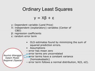
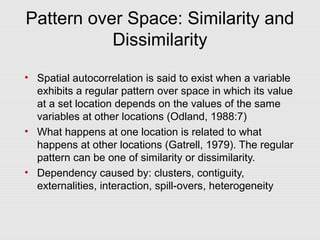
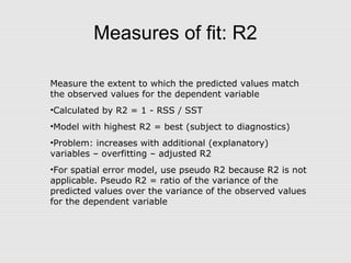
• Value typically range between 0 and 2
• If value of any one zone are spatially unrelated to any other zone, the
expected value of C will be 1
• Values less than 1 (between 1 and 2) indicate negative spatial
autocorrelation
• Inversely related to Moran’s I
• Does not provide identical inference because it emphasizes the
differences in values between pairs of observations, rather than the
covariation between the pairs.
• Moran’s I gives a more global indicator, whereas the Geary
coefficient is more sensitive to differences in small neighborhoods.
∑ ∑
∑ ∑
−
−−
=
i j iij
i j jiij
XXW
XXWN
C 2
2
)((2
])()[1[(](https://image.slidesharecdn.com/ekreg-ho-11-spatialec231112-130909102916-/85/Ekreg-ho-11-spatial-ec-231112-16-320.jpg)
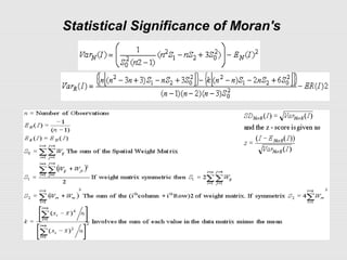
![Expected Value and Variance
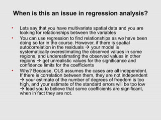
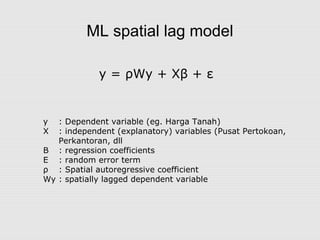
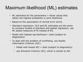
• Expected Value
• Variance
• Statistical Significance
E I
N
S
tr
M
N K
( ) =
−
V I
N
S
tr MWMW tr MW
N K N K E I
( ) .
. ' ( . )
( )( ) [ ( )]
=
+
− − + −
2 2
2
2
M I X X X= − −( ' ) '
Z I
I E I
V I
( )
( )
( )
=
−](https://image.slidesharecdn.com/ekreg-ho-11-spatialec231112-130909102916-/85/Ekreg-ho-11-spatial-ec-231112-17-320.jpg)

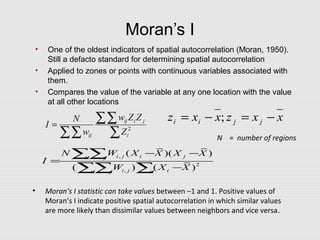
This document discusses spatial econometrics and issues that can arise when performing regression analysis on spatial data. Ordinary least squares (OLS) regression may produce misleading results if there is spatial autocorrelation in the data. Spatial autocorrelation occurs when the value of a variable at one location is influenced by or correlated with values at nearby locations. This can violate OLS assumptions of independent errors. The document describes techniques like Moran's I and Lagrange multiplier tests to detect spatial autocorrelation and spatial regression models like spatial lag and spatial error models that account for spatial effects.