This document contains a student's assignment responses for a solar cell fabrication course. It includes 5 worked problems related to topics like solar cell operation, alkali etching, impurity segregation during crystallization, and diffusion. For each problem, the student provides calculations and analyses to estimate values, predict outcomes, and solve related issues given data and process parameters. Overall, the document demonstrates the student's understanding of key science and technology concepts behind solar cell fabrication.

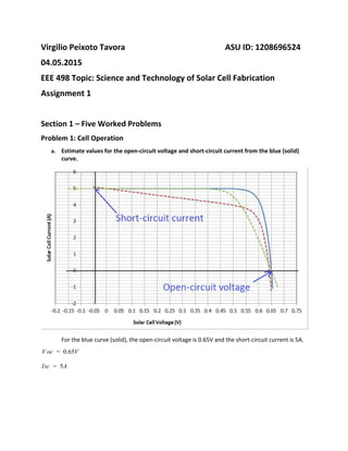
1. Virgilio Peixoto Tavora ASU ID: 1208696524
04.05.2015
EEE 498 Topic: Science and Technology of Solar Cell Fabrication
Assignment 1
Section 1 – Five Worked Problems
Problem 1: Cell Operation
a. Estimate values for the open-circuit voltage and short-circuit current from the blue (solid)
curve​.
For the blue curve (solid), the open-circuit voltage is 0.65V and the short-circuit current is 5A.
oc 0.65VV =
sc 5AI =

2. b. Estimate values for the maximum-power voltage and maximum-power current from the
blue (solid) curve.
the blue curve (solid), the maximum-power voltage is 0.55V and the maximum-power current
is 4.9A.
mp 0.55VV =
mp 4.9AI =
c. Estimate values for the maximum power and fill factor from the blue (solid) curve.
Maximum power = =mpx V mp I .9A x 0.55V4
Maximum power = 2.695 W
Fill Factor = =Isc x V oc
Imp x V mp
5 x 0.65
4,9 x 0.55
Fill Factor = 0.8292 or 82.92%

3. d. Indicate which of the dash curves represents a solar cell with a high series resistance.
green dash curve represents a solar cell with a high series resistance, because it `steals`
voltage depending on the current.
e. Indicate with of the dashed curves represents a solar cell with a low shunt resistance.
red dash curve represents a solar cell with a high series resistance, because it `steals` current
depending on the voltage.
Problem 2: Cell Operation
Voltage (V) Current (A) Note
0.000 5​.400 Short Circuit
0.100 5.368
0.200 5.336
0.300 5.305
0.400 5.272
0.500 5.225
0.570 4.985 Max Power
0.600 4.461
0.650 0.000 Open Circuit
Equation for the IV terminal characteristics of a solar cell given in lecture
a. Using the data in the table above, determine the Voc, Isc, Vmp, Imp, Pmp, FF and efficiency
of the solar cell.
From the table:
andoc 0.65 VV = sc 5.4 AI =
For the maximum power:
andmp 0.57 VV = mp 4.985 AI =

4. = = 2.89145 Wower maximumP mp x ImpV
= =F F Isc x V oc
Imp x V mp
.8095 or 80.95%0
b. Using the data in the table above, estimate the value of ​IL ​for the equation of the IV
terminal characteristics.
≈ I .4 A IL SC = 5
c. c. Using the data in the table above, estimate the value of ​RSH ​for the equation of the IV
terminal characteristics.
sh ≈1 x 10 ohms cmR 3 2
d. d. Using the data in the table above, estimate the value of ​I0 ​for the equation of the IV
terminal characteristics.
≈ 1 x 10 AI0
−3
e. Using​​the data in the table above, estimate the value of ​RS ​for the equation of the IV
terminal characteristics.
.5 Rs .3 ohms cm 0 < < 1 2
f. ​Using your estimates for the values of ​IL​, ​RSH​, ​I0​, and ​RS​, plot the IV terminal characteristics
using Excel or other spreadsheet/plotting software. Double check that your plotted curve
aligns up with the data in the table above!

5. Problem 3: Alkali Etching

6. The current process recipe has a NaOH concentration of 20% and an etch time of 30 minutes.
a. For the current process recipe, how much silicon is etched from each side of the
wafer?
For 20% of NaOH concentration, the Silicon Etch Rate is 55 microns/hour.
Considering an etch time of 30 minutes for both sides of the wafer, the etch time for each side of the
wafer is 15 minutes.
for each side of the wafer, the etched silicon is 13.75 microns. For both sides of the wafer, the
etched silicon is 27.5 microns.
b. If the wafer starting thickness is 220 microns, what is the wafer thickness after the etching
process? NOTE: both sides will be etching during the etch process.
Wafer starting thickness = 220 microns
Wafer starting thickness after the etching process in both sides of the wafer
= 220 – 27.5 = 192.5 micron
The new Diamond Wire Sawn Wafers require 20 microns of silicon to be etched from each side of
the wafer.
c. Predict the etch time that would be required for these wafers, if NaOH concentration was
kept fixed at 20%?
Silicon to be etched = 20 microns for each side of the wafer
For 20% NaOH concentration, the Silicon Etch Rate is 55 microns/hour.
55 microns in 60 minutes
20 microns in X minutes
So, 20 microns of Silicon are etched in 21.81 minutes or 21 minutes and 49 seconds. Both sides of the
wafer are etched in 43.62 minutes or 42 minutes and 37 seconds.
d. Predict the smallest NaOH concentration that would be required for these wafers, if time
was kept fixed at 30 minutes?
20 microns of Silicon to be etched in 30 minutes.
Silicon Etch Rate = 40 microns/hour
Choosing one point before and one point after the Silicon Etch Rate of the case, the equation of the
line was found:
Point 1: (0 microns/hour, 0 %)
Point 2: (48 microns/hour, 10 %)

7. a x X b Y = +
a x 0 b 0 = +
0 b =
8 a x 10 4 =
4.8 a =
Point in the case: (40 microns/hour, X %)
0 4.8 x X 0 4 = +
of NaOH concentration 8.33% X =
e. Management wants the process to run faster. Predict the NaOH concentration that would
be required for these wafers, if a process time of 15 minutes was required.
f. Part e presents an interesting situation. Make one suggestion about what other things the
engineering team might do to change the alkali etching process recipe in order to address
this interesting situation.
Problem 4: Segregation of Impurities during Crystallization of Silicon
Impurit
y
Al As B C Cu Fe O P Sb
k0 0.002 0.3 0.8 0.07 4x10-6 8x10-6 0.25 0.35 0.023
a. Chunk poly silicon has an iron impurity concentration of 1 part per million iron atomic
(ppma) in silicon. Determine the iron impurity concentration (in ppma) in the molten silicon
during Czochralski ingot growth. Determine the iron impurity (in ppma) in the solidified
silicon ingot during Czochralski ingot growth.
b. Three grades of chunk poly silicon are listed in the table below. Which are suitable for SG-Si
grade of wafers, if any? NOTE: refer to Slide 5 in Lecture 3 for the specification for SG-Si.
ALSO NOTE: the data in the chart and table in the lecture notes on Lecture 3, Slide 5 refers
to the impurity concentrations in the solidified silicon ingot, not in the chunk poly.
Iron (Fe)
(ppmw)
Chromium (Cr)
(ppmw)
Titanium (Ti)
(ppmw)
Copper (Cu)
(ppmw)
Segregation Coefficient
at Growth Conditions 8.00E-06 1.10E-05 1.00E-06 4.00E-04
Chunk Poly #1 2.25E+06 2.00E+05 2.00E+05 2.50E+02
Chunk Poly #2 2.75E+06 1.91E+05 3.80E+05 6.25E+02
Chunk Poly #3 3.50E+06 3.00E+05 4.60E+05 1.38E+03

8. Problem 5: Diffusion
1. The phosphorous source is a vapor of POCl3. First, a pre-deposition step (infinite
diffusion) is performed. Then, the phosphorus source is switched off. Second, a drive-in step
(limited diffusion) is performed.
2. The pre-deposition is performed at 900 degrees C for 30 minutes. Hint: use seconds in the
calculations, not minutes.
3. During the pre-deposition, the surface concentration N0 is given by the solid solubility of
phosphorus. Note: use the “solubility limit” curve, not the “electrically active” curve.
4. The diffusivity of phosphorus is given in a table in the lecture notes.
5. The drive-in is performed at 1000 degrees C for 2 hours. Hint: use seconds, not hours.
6. The background doping concentration is NB = 1x10^16 cm-3
a. Calculate the dose Q for the pre-deposition process. The surface concentration is 5.31e20
atoms/cm3.
5.31 x 10 atoms/cmN0 = 20 3
(at T 900 degrees C ) 1.5 x 10 cm /sD = = −15 2
30 minutes 1800 seconds t = =
(t) 2 N Q = 0√π
Dt
[ ]t 2.7 x 10D = −12
(t) 2 x 5.31 x 10 Q = 20
√ π
2.7 x 10−12
(t) 9.845356861 x 10 atoms/cmQ = 14 2
b. For the drive-in step, write an equation for the concentration of phosphorus atoms at the
surface (ie. x = 0.0 cm) as a function of time.
5.31 x 10 atoms/cmN0 = 20 3
(at T 1000 degrees C ) 2.6 x 10 cm /sD = = −14 2
2 hours 20 minutes 7200 seconds t = = 1 =
(t) 9.845356861 x 10 atoms/cmQ = 14 2
(x, ) . exp⁡[− ] N t = Q
√Dtπ
( )x
2√Dt
2
x = 0.0 cm, (0, ) . exp⁡[0] N t = 9.845356861 x 1014
√2.6 x 10 x π x t−14
(0, ) . 1 N t = 2.858 x 10 −7 √t
9.845356861 x 1014

9. (0, ) atoms/cmN t = √t
3.445 x 1021
3
c. Calculate the concentration of phosphorus atoms at the surface at the end of the drive in
step. Hint: it will be lower than the surface concentration you used in (a) above.
t = 2 hours = 120 minutes = 7200 seconds
(0, ) N t = √t
3.445 x 1021
(0, 200) N 7 = √7200
3.445 x 1021
(0, 200) 4.059971435 x 10 atoms/cmN 7 = 19 3
d. ​Calculate the junction depth at the end of the drive in step ​in microns​. Note: the unit of xj
given in the lecture notes is cm.
5.31 x 10 atoms/cmN0 = 20 3
1 x 10 atoms/cmNB = 16 3
t .872 x x 10D = 1 −10
Junction Depth x j
2 x j =
√Dt ln( )NB
N0
2 x j = √1.872 x x 10 x (10.87993221)−10
2 x 4.513007107 x 10 x j = −5
9.026014202 x 10 cm x j = −5
0.9026014202 microns x j =