This document provides an introduction to statistics and data collection methods. It discusses key concepts such as:
1. The difference between economic and non-economic activities, and definitions of common economic roles like consumers, producers, service holders and service providers.
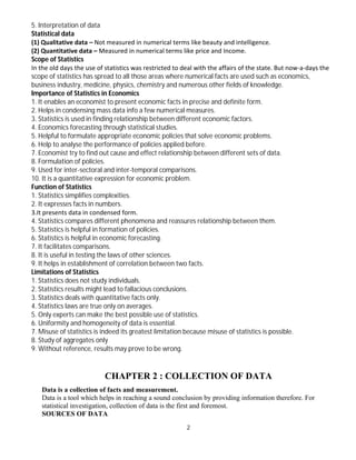
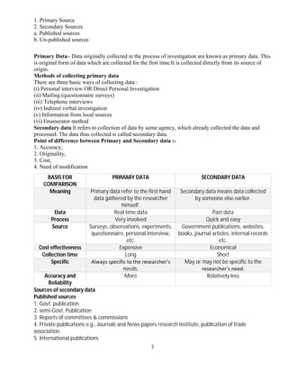
2. The stages of collecting statistical data, including primary and secondary sources, methods of collecting primary data, and the differences between primary and secondary data.
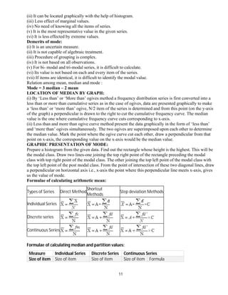
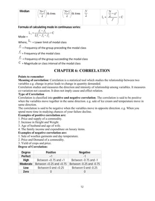
3. Methods of organizing raw data through classification, frequency distributions, and other statistical techniques. Common approaches to presenting organized data are also outlined, including tables, diagrams and graphs.
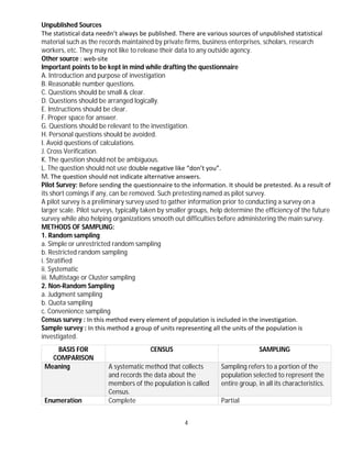
4. Sampling methods like census surveys and sample surveys are introduced, along with the differences between them. Key organizations involved in