Communication System
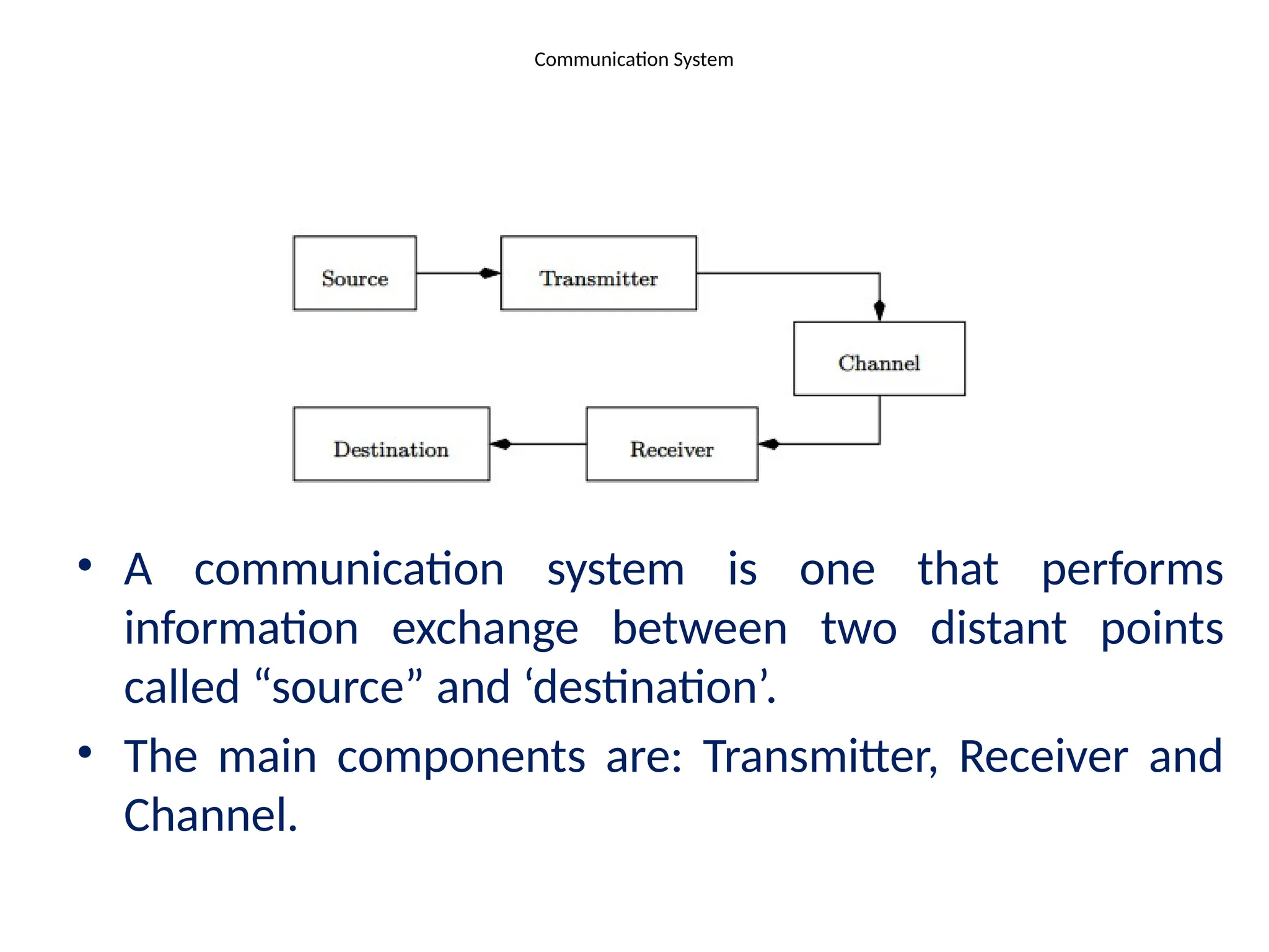
• Acommunication system is one that performs
information exchange between two distant points
called “source” and ‘destination’.
• The main components are: Transmitter, Receiver and
Channel.
3.
• The transmitterconverts the information signal into a
form that is suitable for transmission through
channel.
• Channel provides medium of information
transmission to the receiver and may be wire-line or
wireless (radio).
• A receiver performs the recovery of information
signal at destination.
• The source of information is usually voice, pictures,
computer data etc.
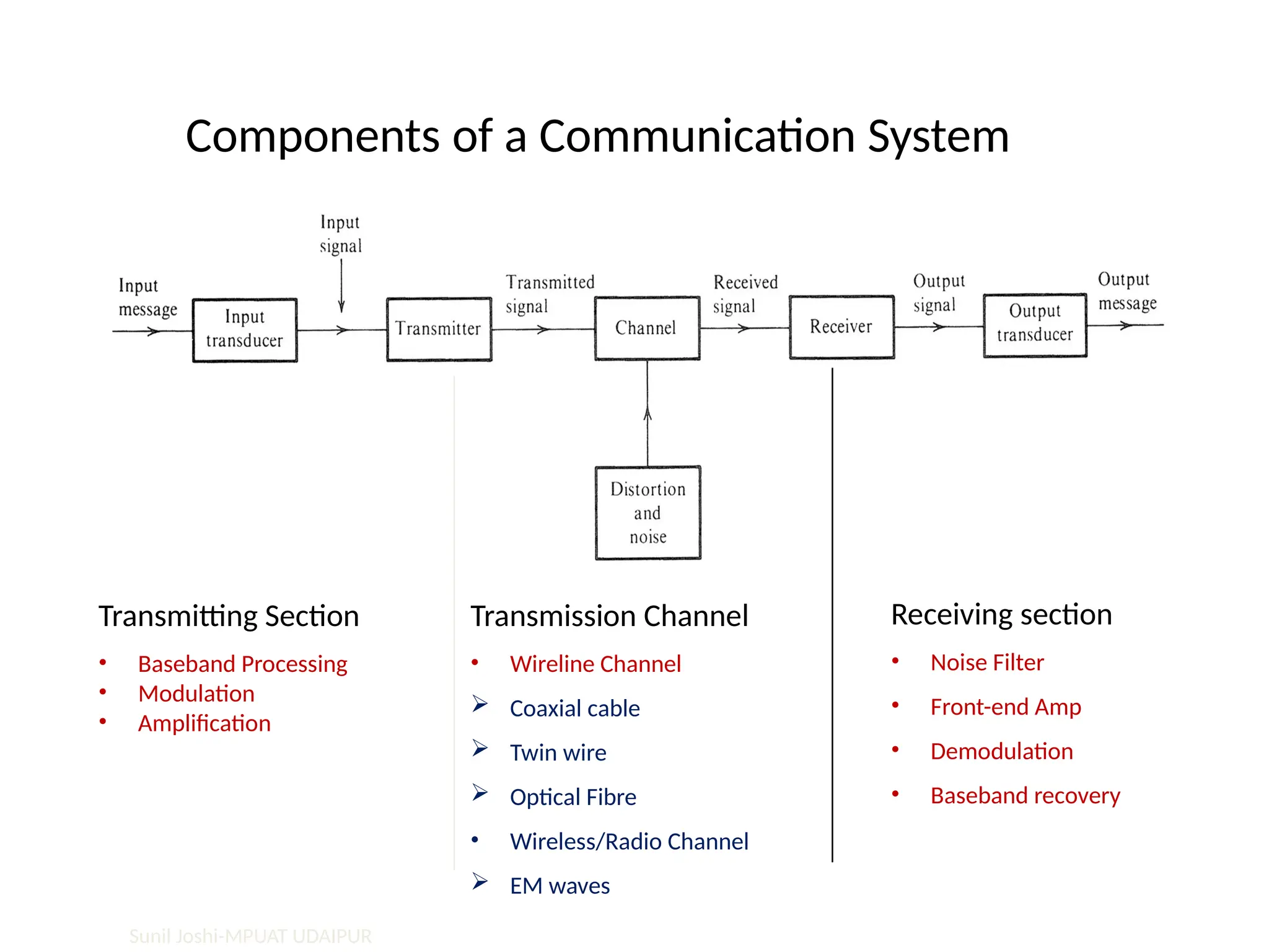
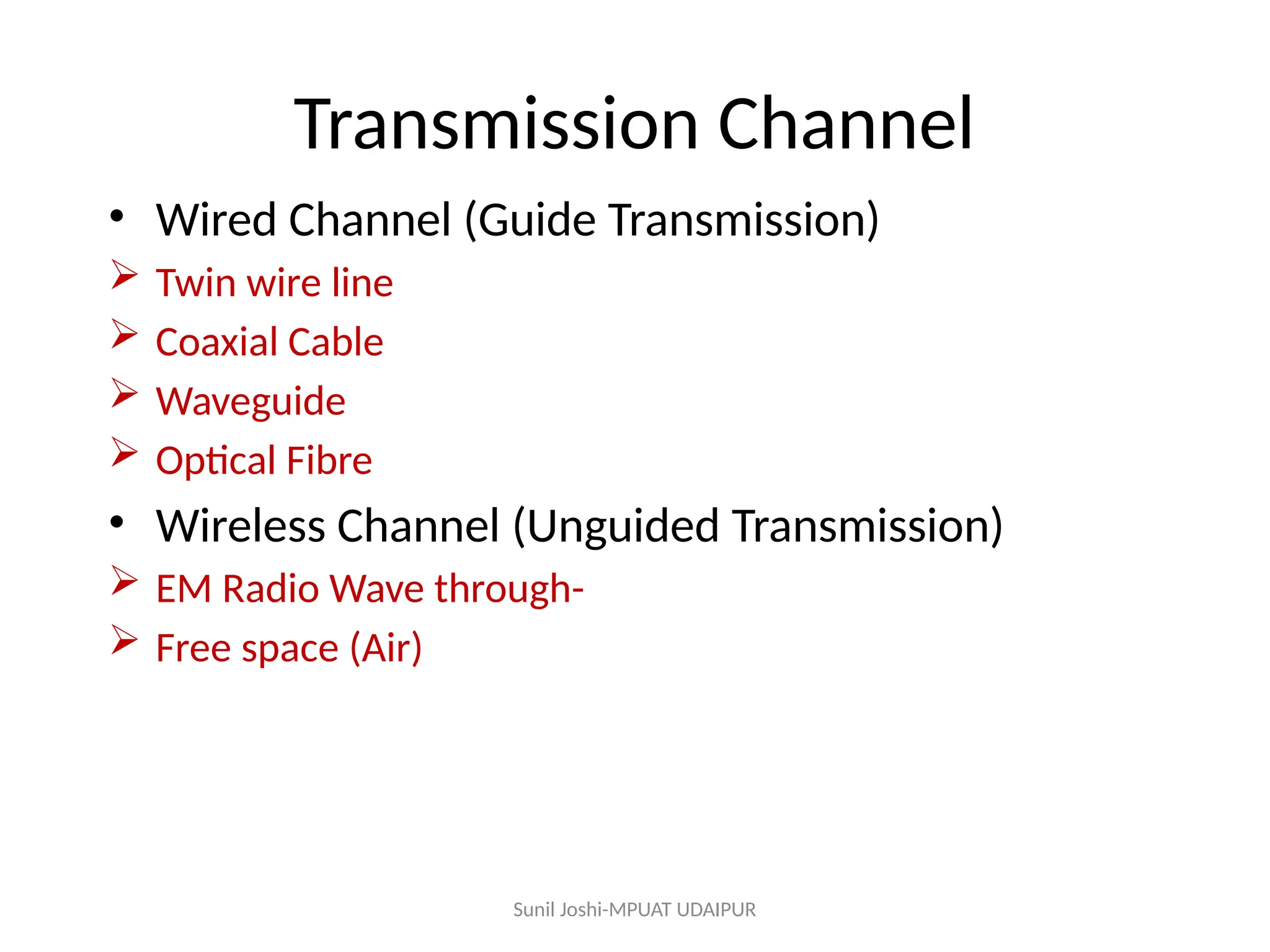
Transmission Channel
• WiredChannel (Guide Transmission)
Twin wire line
Coaxial Cable
Waveguide
Optical Fibre
• Wireless Channel (Unguided Transmission)
EM Radio Wave through-
Free space (Air)
Sunil Joshi-MPUAT UDAIPUR
7.
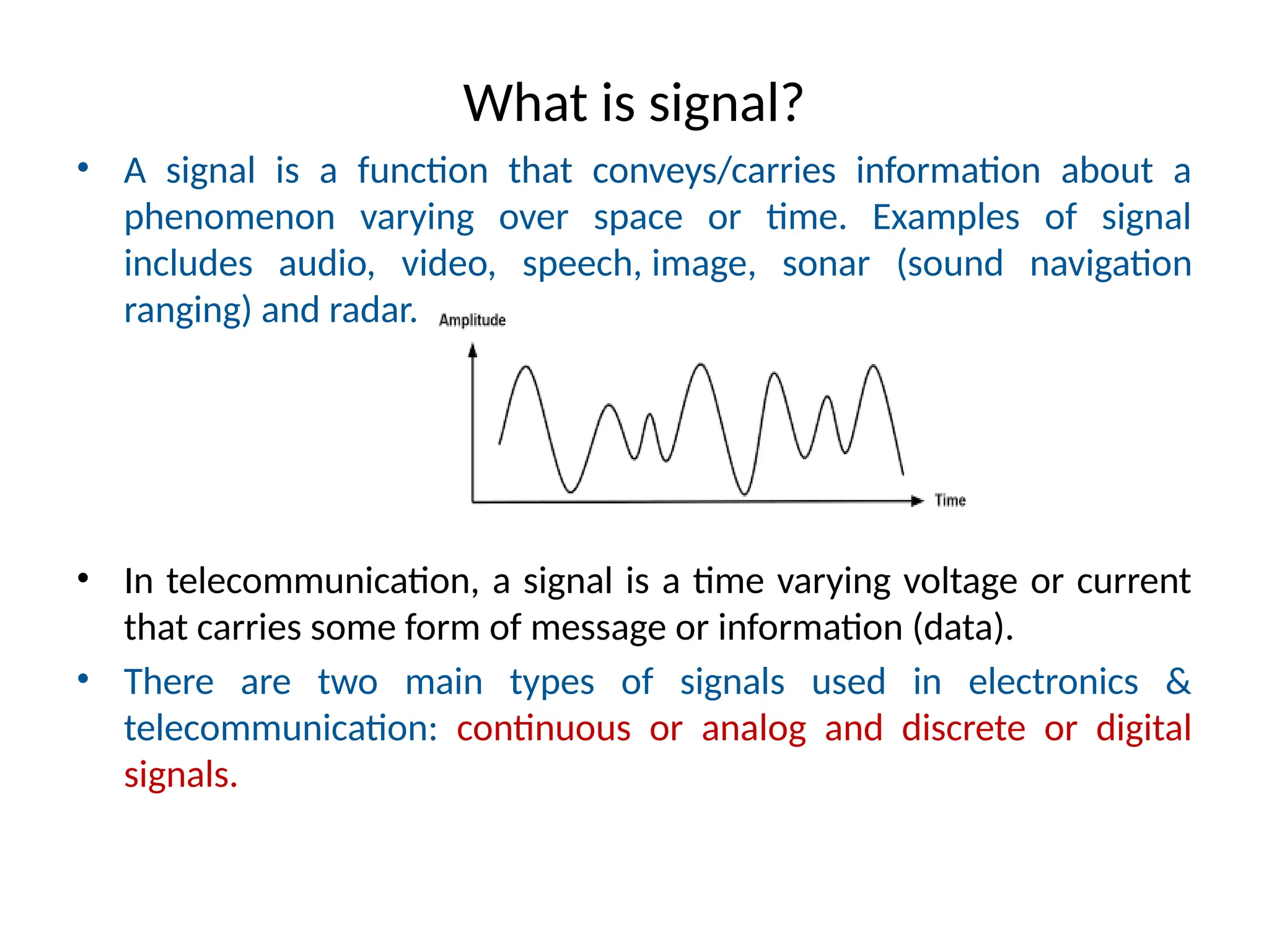
What is signal?
•A signal is a function that conveys/carries information about a
phenomenon varying over space or time. Examples of signal
includes audio, video, speech, image, sonar (sound navigation
ranging) and radar.
• In telecommunication, a signal is a time varying voltage or current
that carries some form of message or information (data).
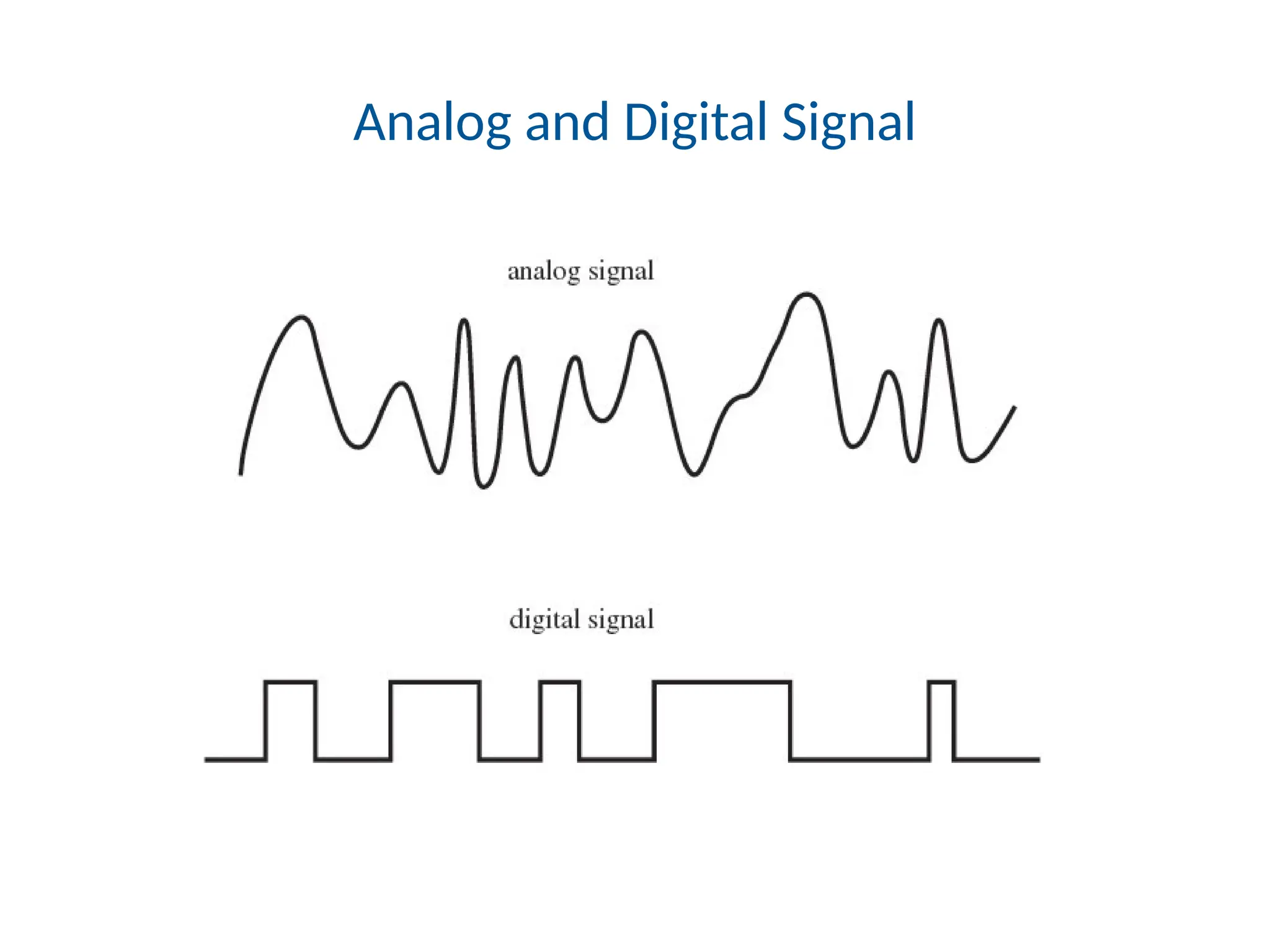
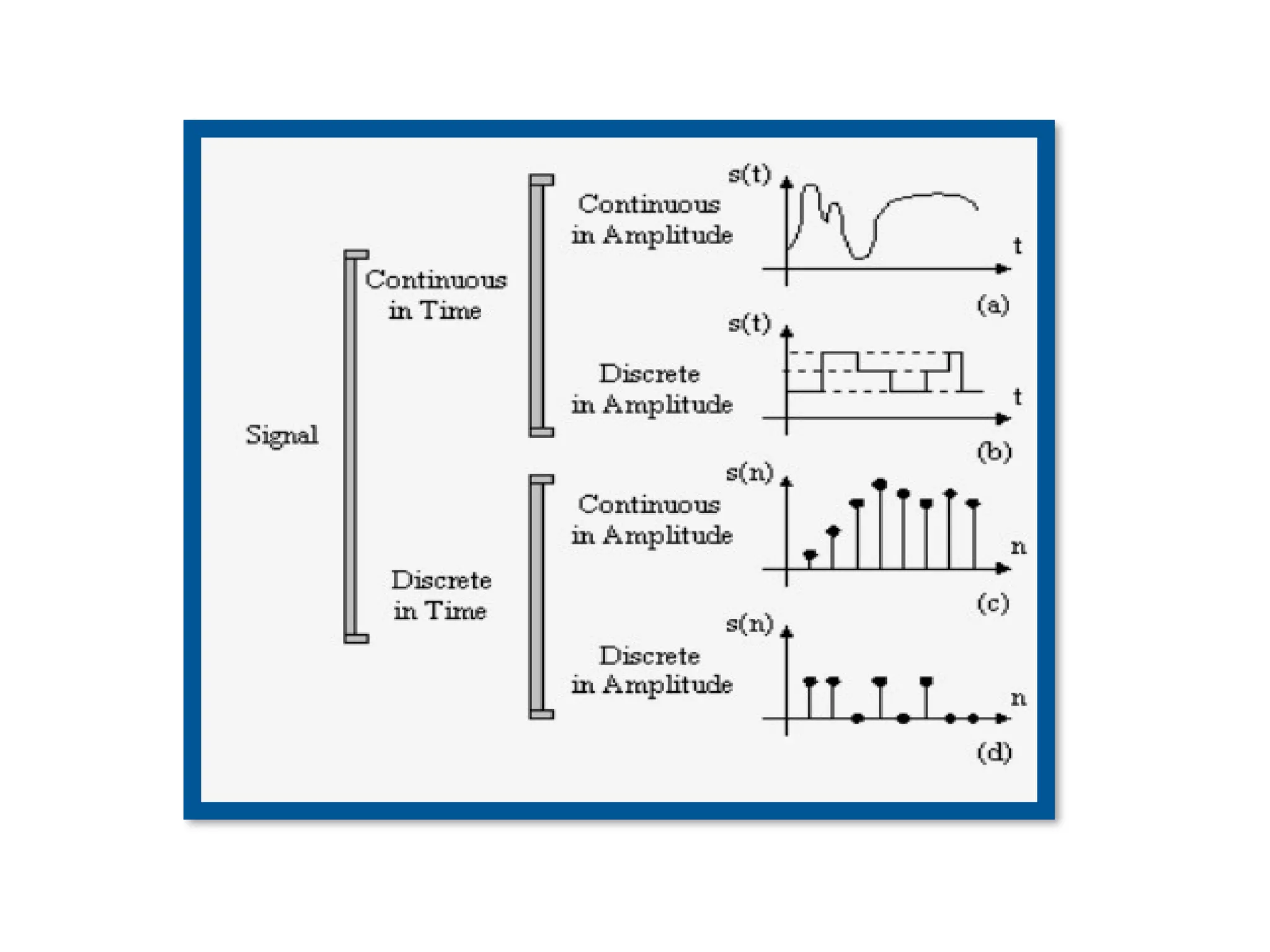
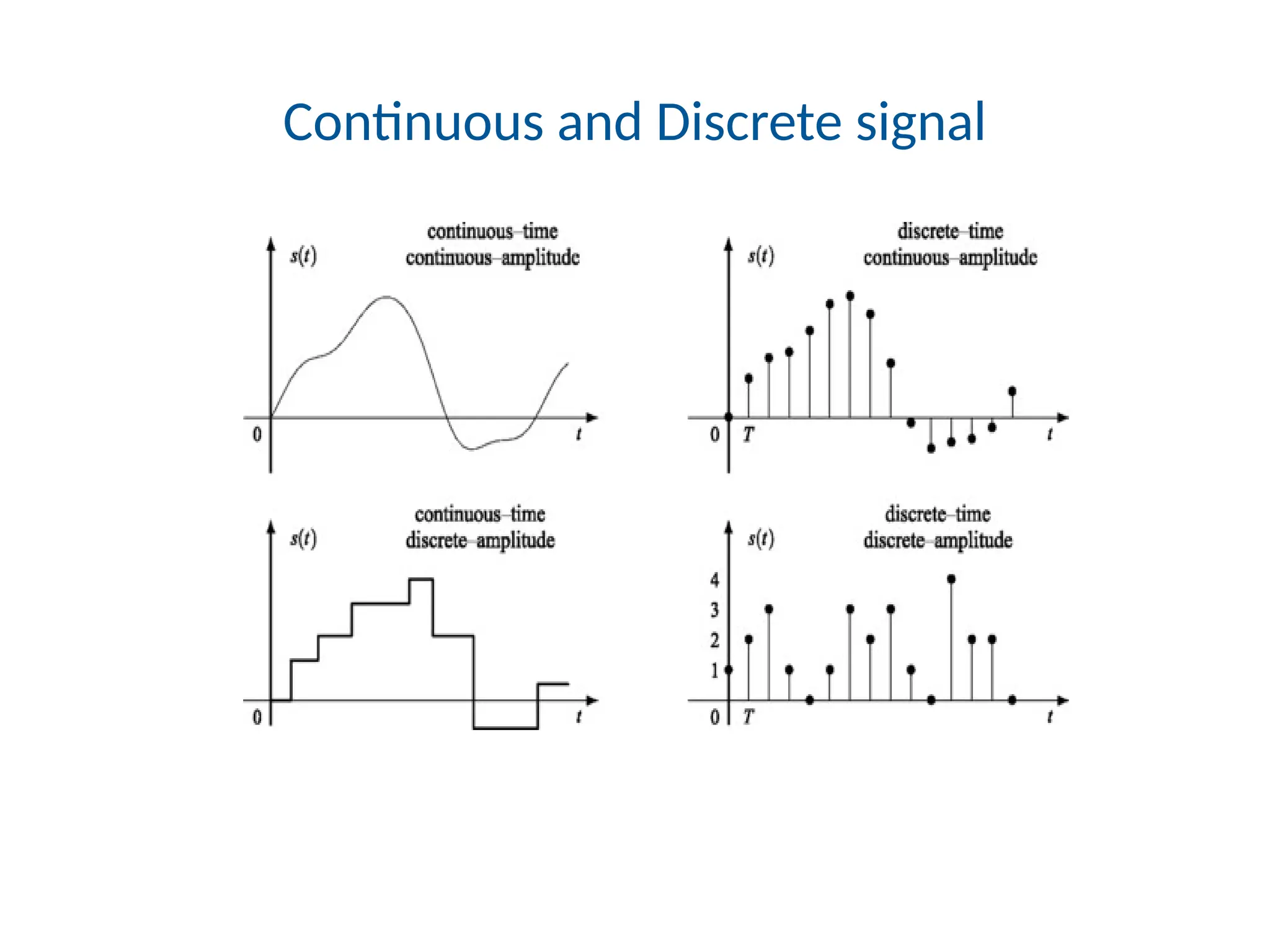
• There are two main types of signals used in electronics &
telecommunication: continuous or analog and discrete or digital
signals.
8.
Signal definitions
• Inelectronics and telecommunications, signal refers to any
time-varying voltage, current, or electromagnetic wave that
carries information.
• In signal processing, signals are analog and digital
representations of analog physical quantities.
• In information theory, a signal is a codified message, that is, the
sequence of states in a communication channel that encodes a
message.
• In a communication system, a transmitter encodes a message to
create a signal, which is carried to a receiver by the
communication channel.
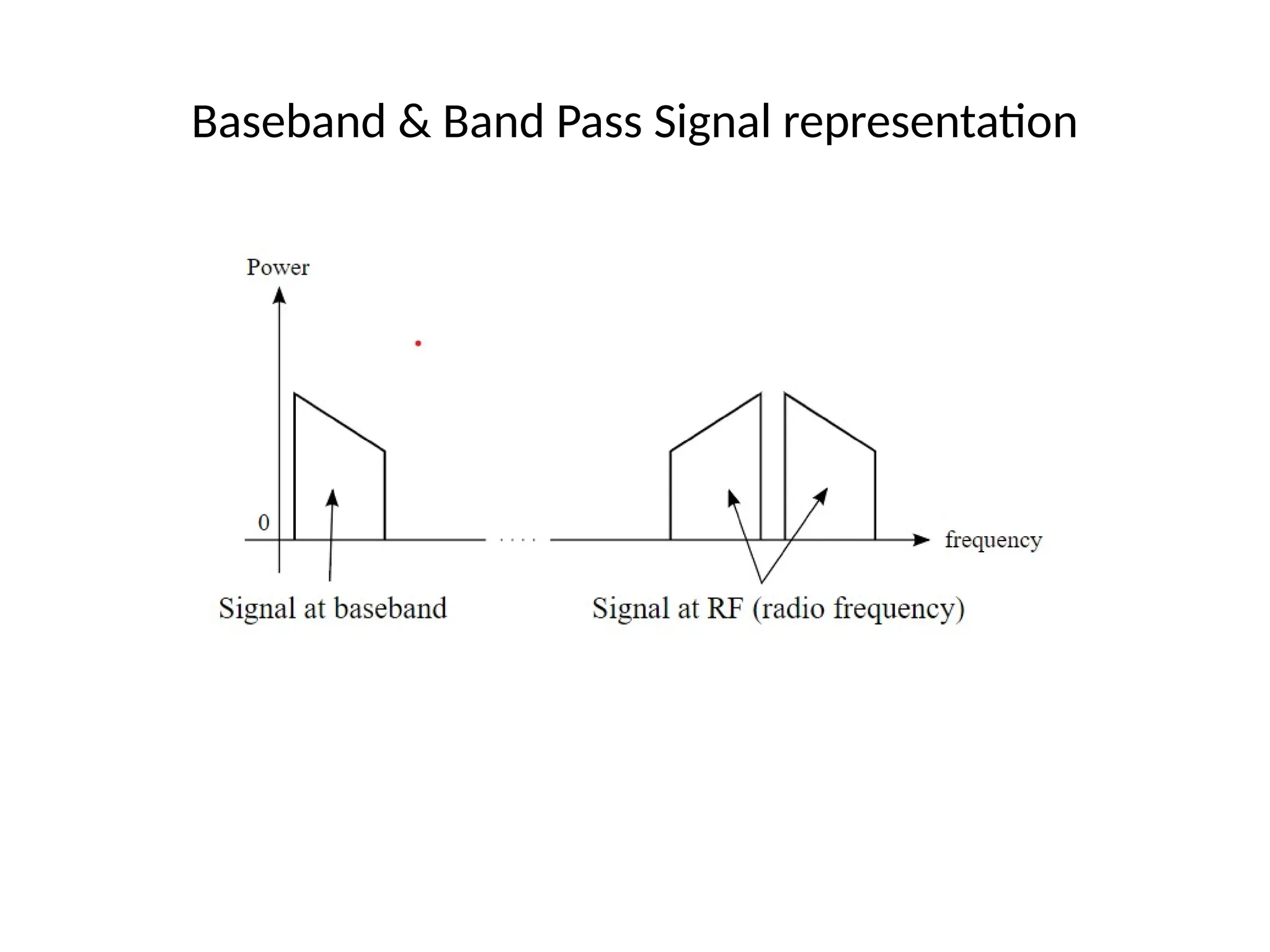
Baseband Signal
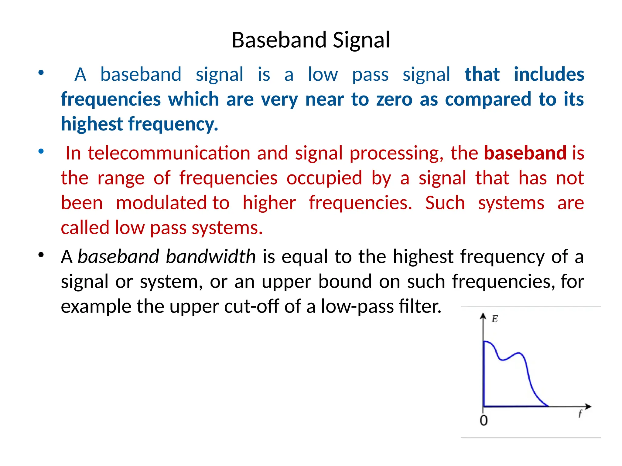
• Abaseband signal is a low pass signal that includes
frequencies which are very near to zero as compared to its
highest frequency.
• In telecommunication and signal processing, the baseband is
the range of frequencies occupied by a signal that has not
been modulated to higher frequencies. Such systems are
called low pass systems.
• A baseband bandwidth is equal to the highest frequency of a
signal or system, or an upper bound on such frequencies, for
example the upper cut-off of a low-pass filter.
13.
• Baseband signalstypically originate from transducers,
converting some other variable into an electrical signal.
• For example, the output of a microphone is a baseband signal
that is an analog of the applied voice audio.
• A baseband signal may have frequency components going all
the way down to DC, or at least it will have a high ratio
bandwidth.
14.
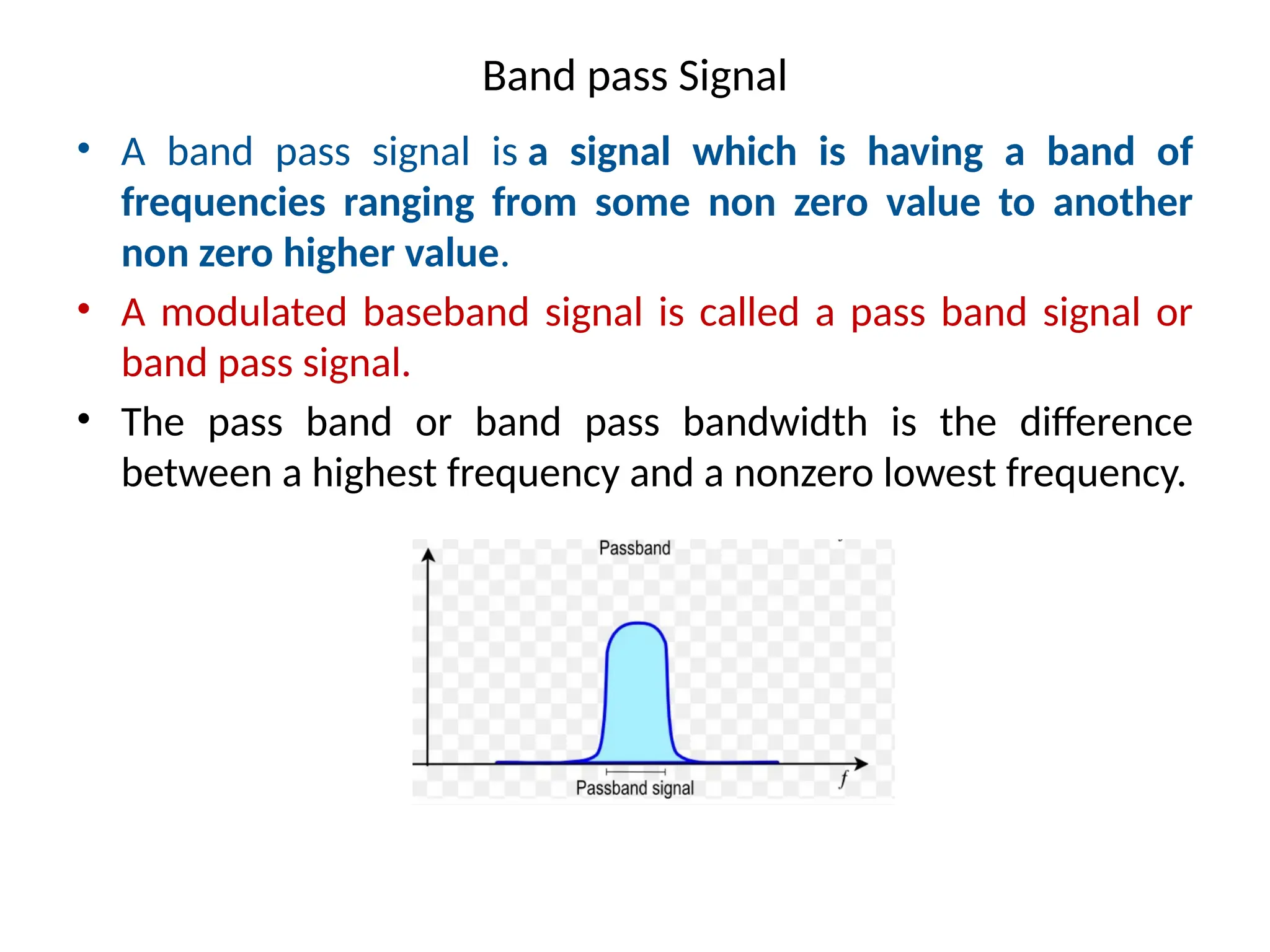
Band pass Signal
•A band pass signal is a signal which is having a band of
frequencies ranging from some non zero value to another
non zero higher value.
• A modulated baseband signal is called a pass band signal or
band pass signal.
• The pass band or band pass bandwidth is the difference
between a highest frequency and a nonzero lowest frequency.
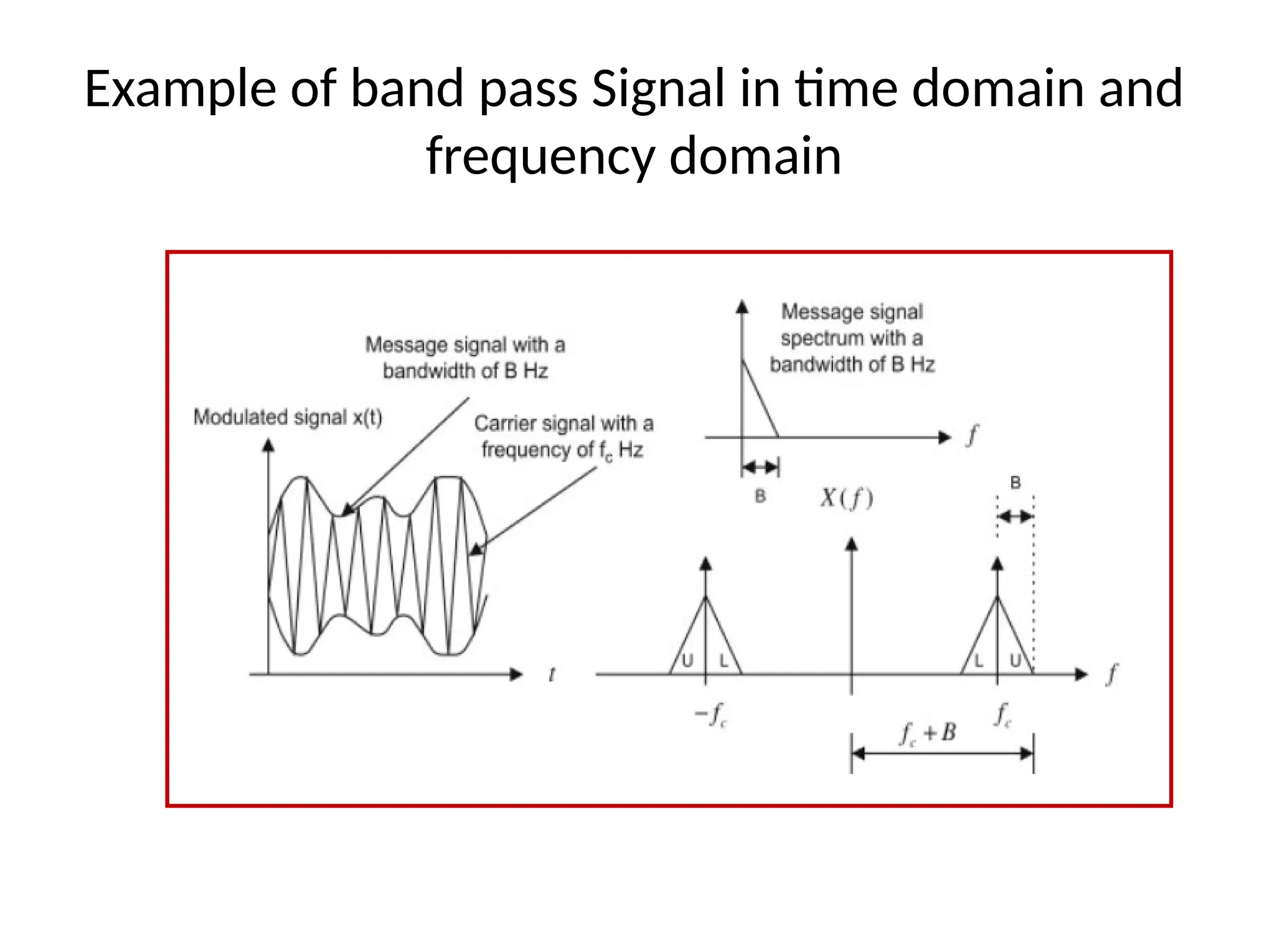
Example of bandpass Signal in time domain and
frequency domain
17.
Baseband channel
• Abaseband channel or low pass channel (or system,
or network) is a communication channel that can transfer
frequencies that are very near zero.
• Examples are serial cables and local area networks (LANs),
as opposed to pass band or band pass channels such as
radio frequency channels and band pass filtered wires of
the analog telephone network.
• Frequency division multiplexing (FDM) allows an analog
telephone wire to carry a baseband telephone call,
concurrently as one or several carrier-modulated
telephone calls.
18.
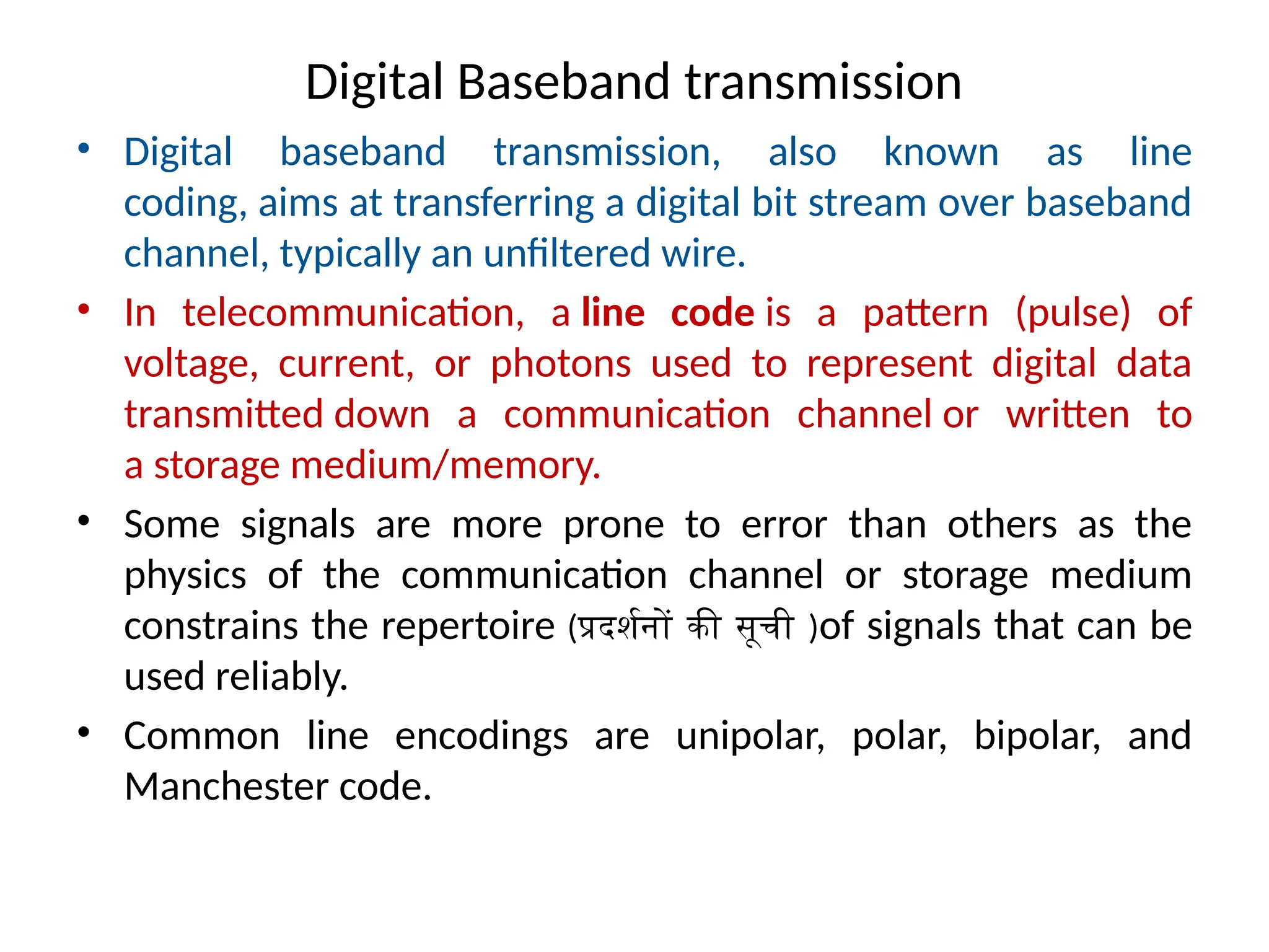
Digital Baseband transmission
•Digital baseband transmission, also known as line
coding, aims at transferring a digital bit stream over baseband
channel, typically an unfiltered wire.
• In telecommunication, a line code is a pattern (pulse) of
voltage, current, or photons used to represent digital data
transmitted down a communication channel or written to
a storage medium/memory.
• Some signals are more prone to error than others as the
physics of the communication channel or storage medium
constrains the repertoire (प्रदर्शनों की सूची )of signals that can be
used reliably.
• Common line encodings are unipolar, polar, bipolar, and
Manchester code.
19.
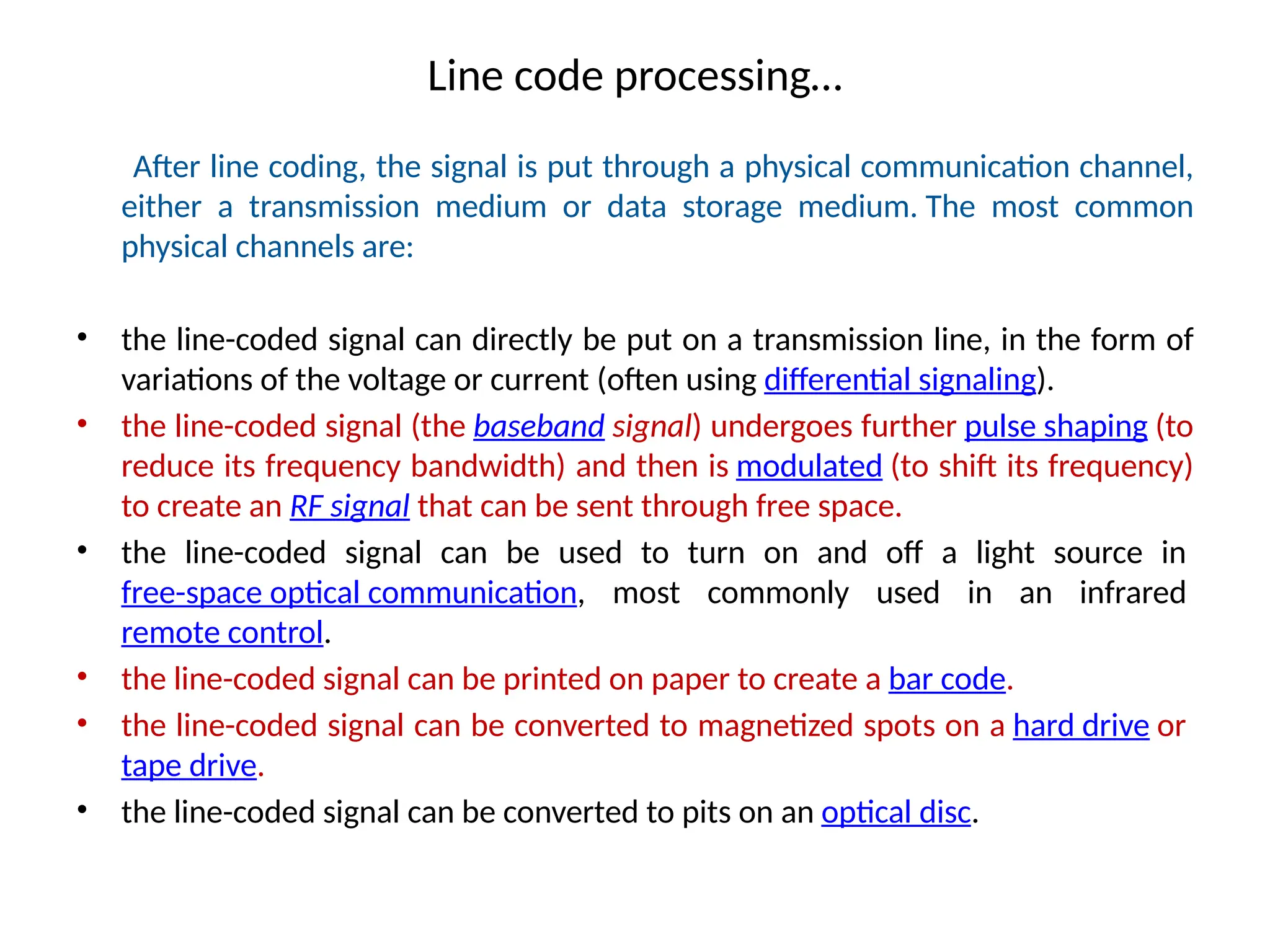
Line code processing…
Afterline coding, the signal is put through a physical communication channel,
either a transmission medium or data storage medium. The most common
physical channels are:
• the line-coded signal can directly be put on a transmission line, in the form of
variations of the voltage or current (often using differential signaling).
• the line-coded signal (the baseband signal) undergoes further pulse shaping (to
reduce its frequency bandwidth) and then is modulated (to shift its frequency)
to create an RF signal that can be sent through free space.
• the line-coded signal can be used to turn on and off a light source in
free-space optical communication, most commonly used in an infrared
remote control.
• the line-coded signal can be printed on paper to create a bar code.
• the line-coded signal can be converted to magnetized spots on a hard drive or
tape drive.
• the line-coded signal can be converted to pits on an optical disc.
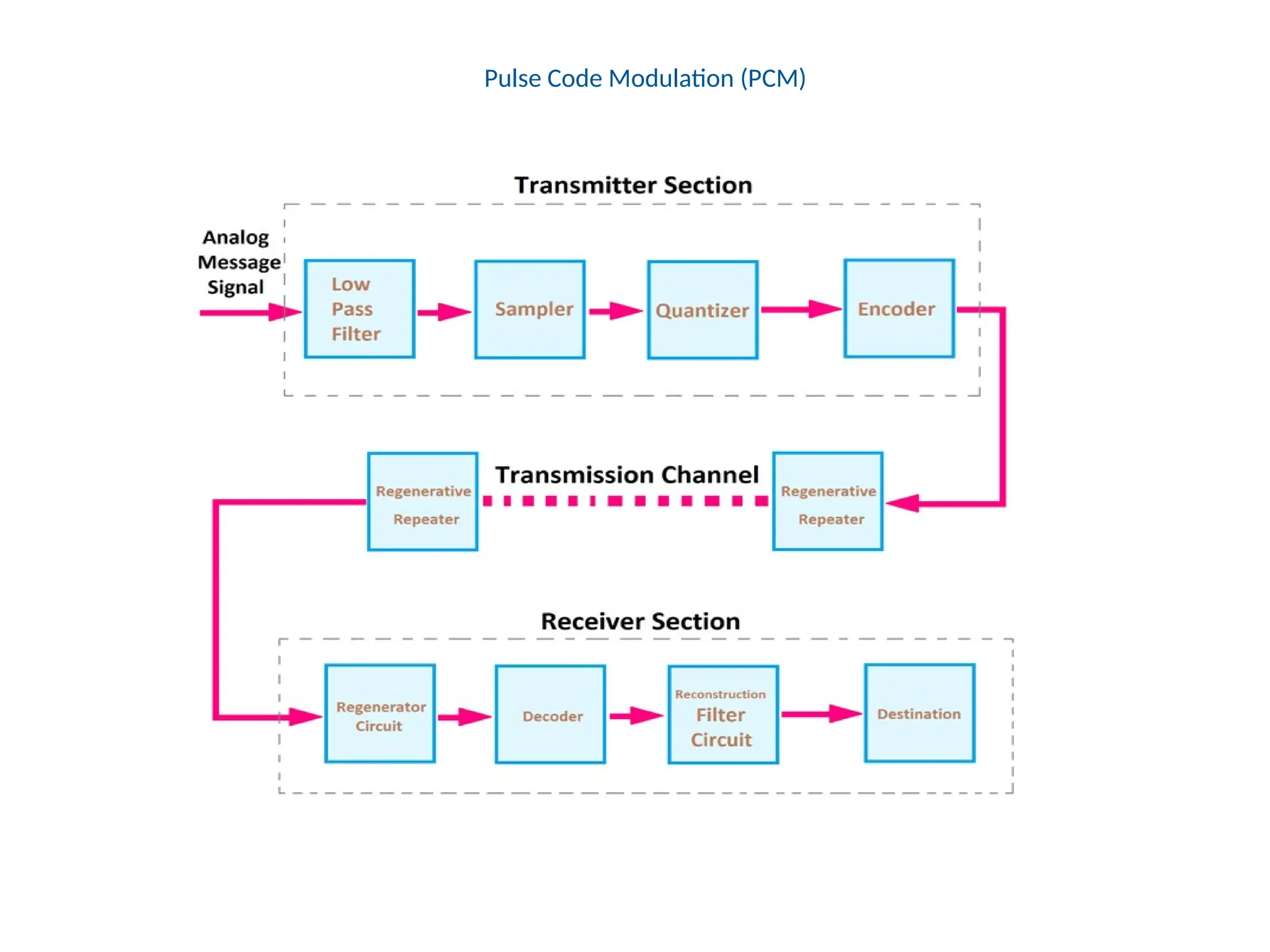
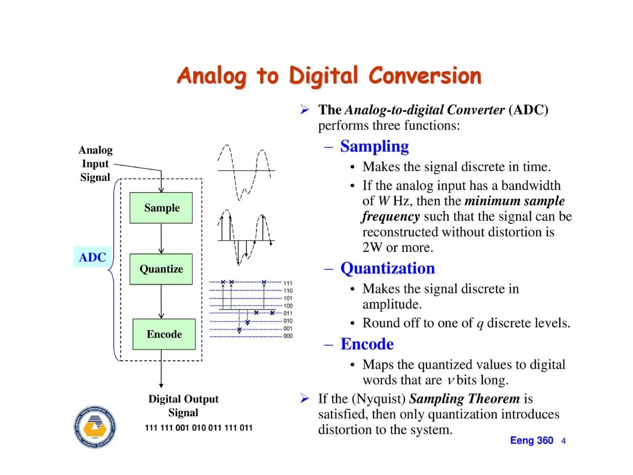
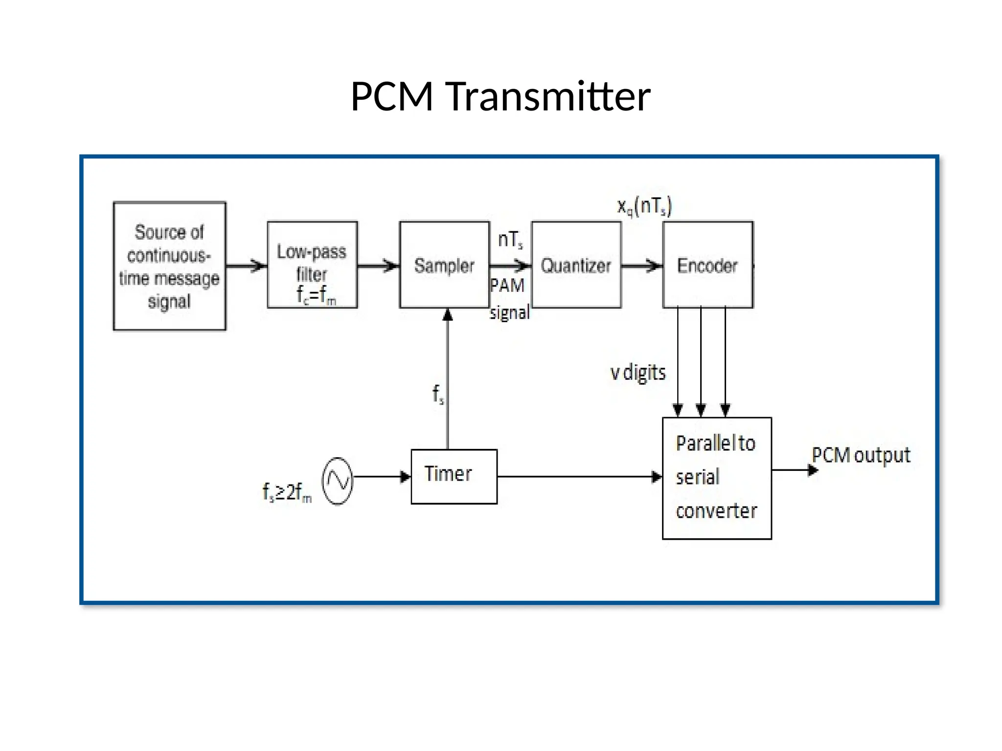
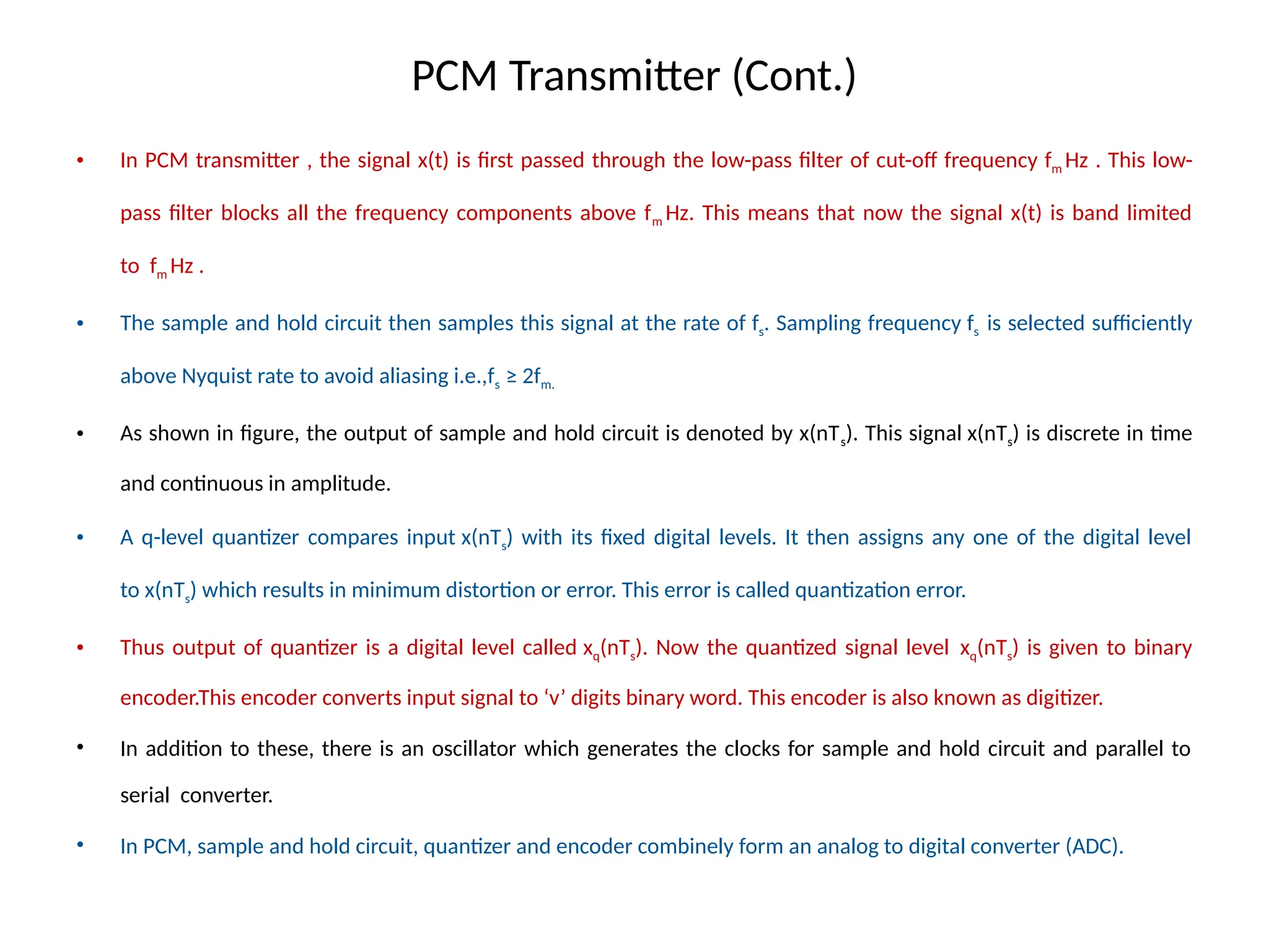
PCM Transmitter (Cont.)
•In PCM transmitter , the signal x(t) is first passed through the low-pass filter of cut-off frequency fm Hz . This low-
pass filter blocks all the frequency components above fm Hz. This means that now the signal x(t) is band limited
to fm Hz .
• The sample and hold circuit then samples this signal at the rate of fs. Sampling frequency fs is selected sufficiently
above Nyquist rate to avoid aliasing i.e.,fs ≥ 2fm.
• As shown in figure, the output of sample and hold circuit is denoted by x(nTs). This signal x(nTs) is discrete in time
and continuous in amplitude.
• A q-level quantizer compares input x(nTs) with its fixed digital levels. It then assigns any one of the digital level
to x(nTs) which results in minimum distortion or error. This error is called quantization error.
• Thus output of quantizer is a digital level called xq(nTs). Now the quantized signal level xq(nTs) is given to binary
encoder.This encoder converts input signal to ‘v’ digits binary word. This encoder is also known as digitizer.
• In addition to these, there is an oscillator which generates the clocks for sample and hold circuit and parallel to
serial converter.
• In PCM, sample and hold circuit, quantizer and encoder combinely form an analog to digital converter (ADC).
Transmission Path orChannel
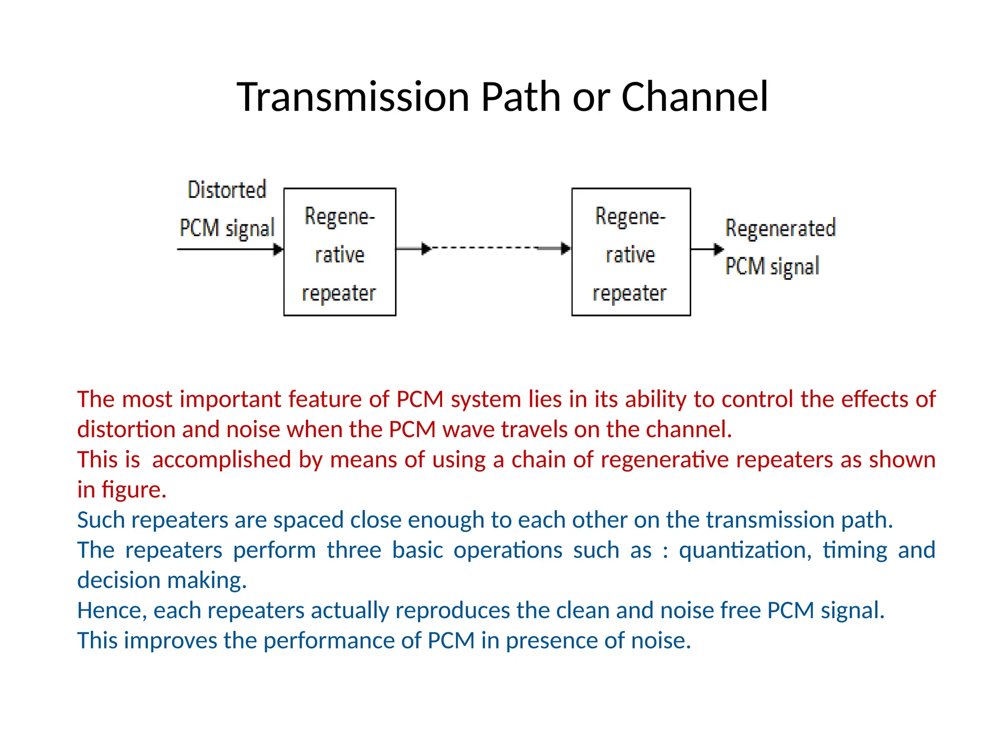
The most important feature of PCM system lies in its ability to control the effects of
distortion and noise when the PCM wave travels on the channel.
This is accomplished by means of using a chain of regenerative repeaters as shown
in figure.
Such repeaters are spaced close enough to each other on the transmission path.
The repeaters perform three basic operations such as : quantization, timing and
decision making.
Hence, each repeaters actually reproduces the clean and noise free PCM signal.
This improves the performance of PCM in presence of noise.
27.
Regenerative Repeater
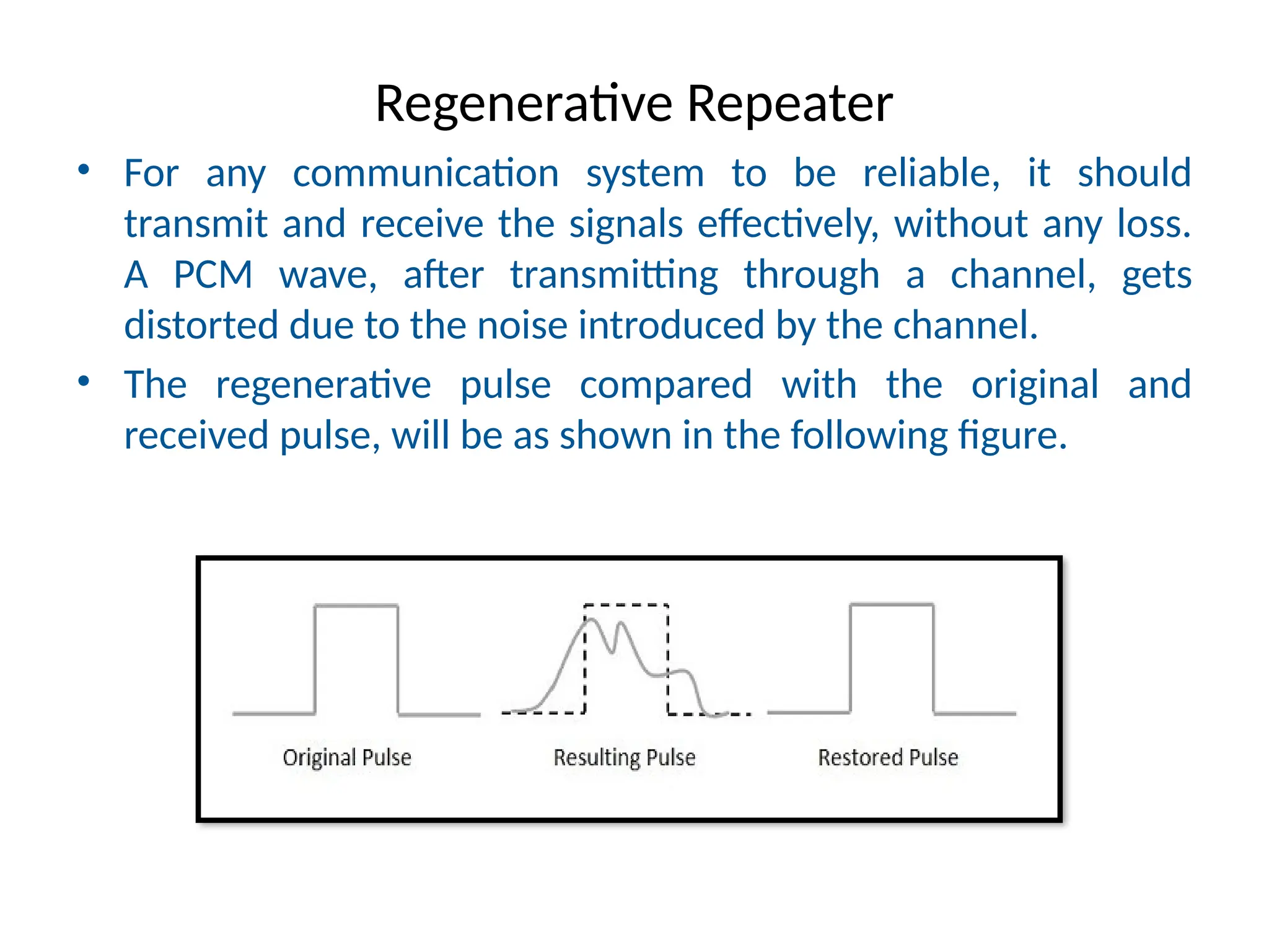
• Forany communication system to be reliable, it should
transmit and receive the signals effectively, without any loss.
A PCM wave, after transmitting through a channel, gets
distorted due to the noise introduced by the channel.
• The regenerative pulse compared with the original and
received pulse, will be as shown in the following figure.
28.
Regenerative Repeater (cont.)
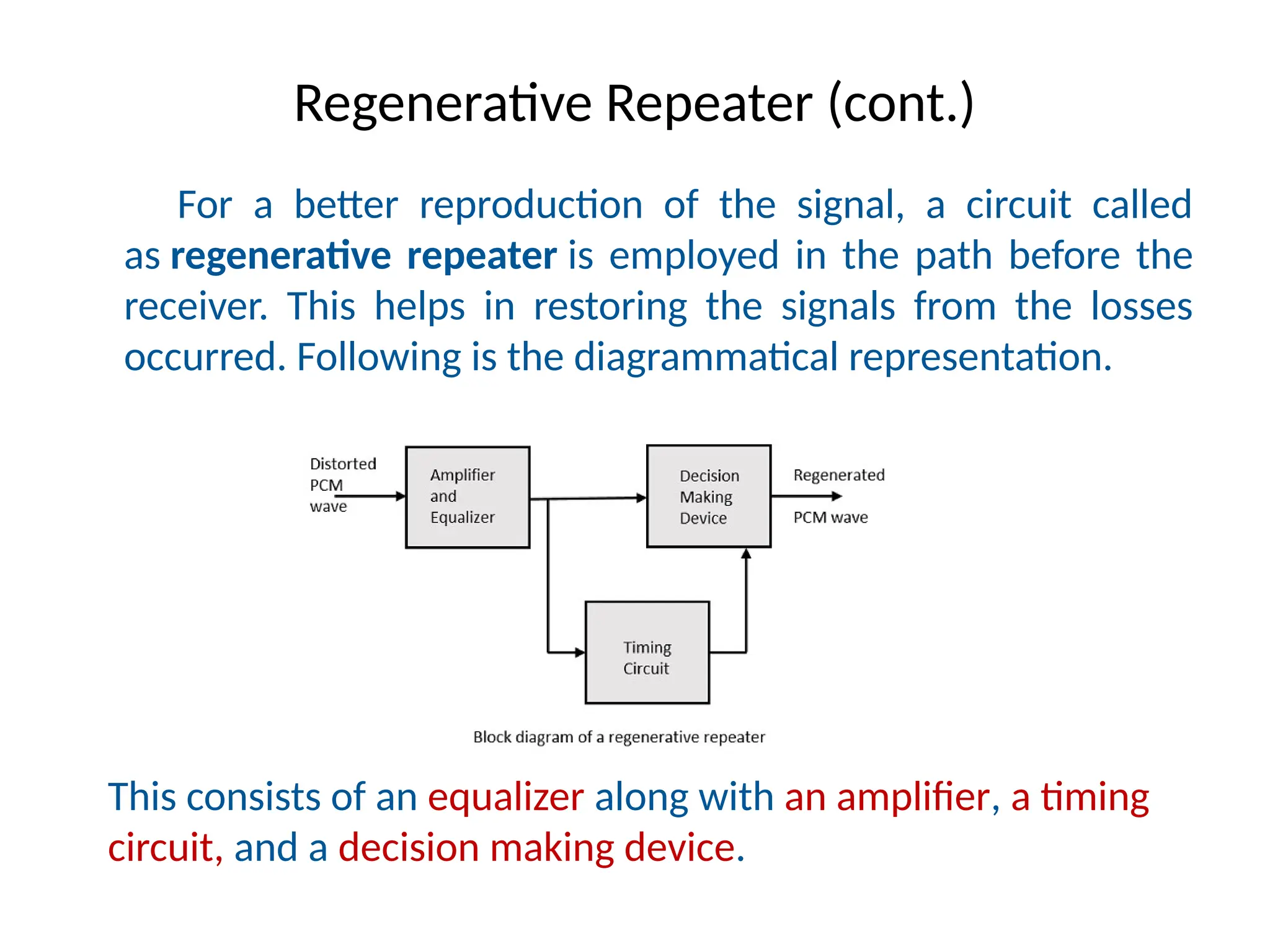
Fora better reproduction of the signal, a circuit called
as regenerative repeater is employed in the path before the
receiver. This helps in restoring the signals from the losses
occurred. Following is the diagrammatical representation.
This consists of an equalizer along with an amplifier, a timing
circuit, and a decision making device.
29.
Regenerative Repeater (cont.)
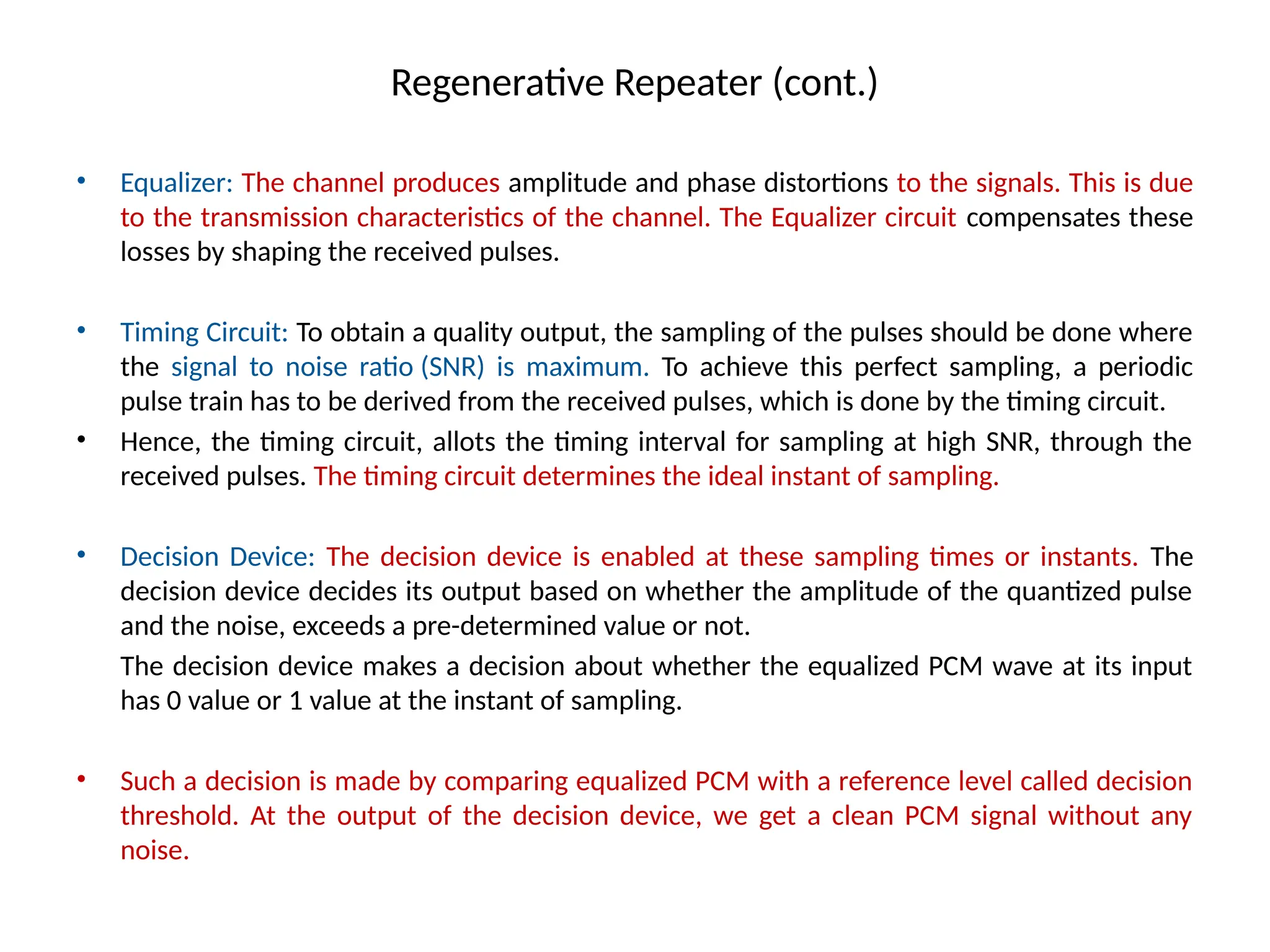
•Equalizer: The channel produces amplitude and phase distortions to the signals. This is due
to the transmission characteristics of the channel. The Equalizer circuit compensates these
losses by shaping the received pulses.
• Timing Circuit: To obtain a quality output, the sampling of the pulses should be done where
the signal to noise ratio (SNR) is maximum. To achieve this perfect sampling, a periodic
pulse train has to be derived from the received pulses, which is done by the timing circuit.
• Hence, the timing circuit, allots the timing interval for sampling at high SNR, through the
received pulses. The timing circuit determines the ideal instant of sampling.
• Decision Device: The decision device is enabled at these sampling times or instants. The
decision device decides its output based on whether the amplitude of the quantized pulse
and the noise, exceeds a pre-determined value or not.
The decision device makes a decision about whether the equalized PCM wave at its input
has 0 value or 1 value at the instant of sampling.
• Such a decision is made by comparing equalized PCM with a reference level called decision
threshold. At the output of the decision device, we get a clean PCM signal without any
noise.
30.
PCM receiver
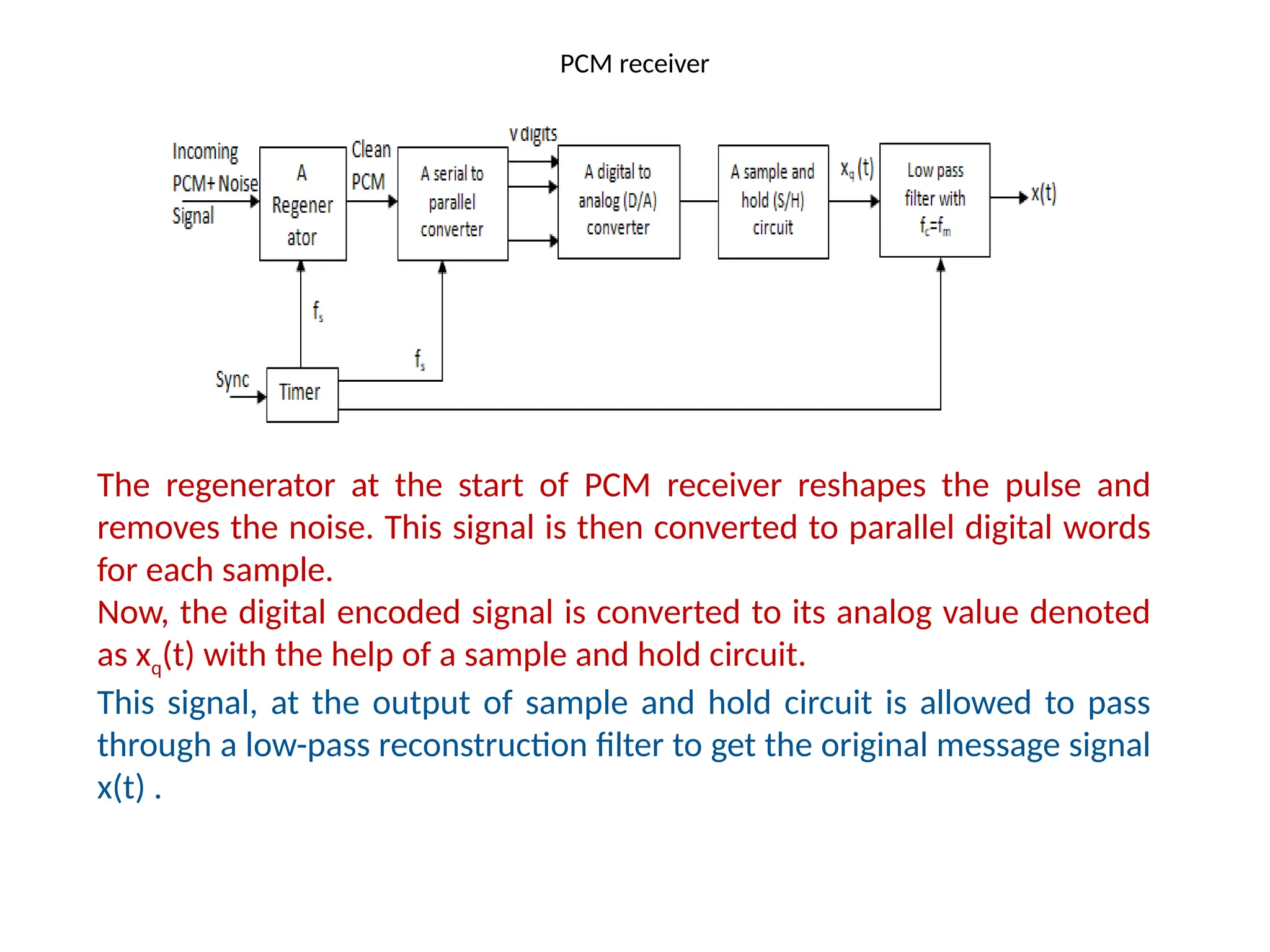
The regeneratorat the start of PCM receiver reshapes the pulse and
removes the noise. This signal is then converted to parallel digital words
for each sample.
Now, the digital encoded signal is converted to its analog value denoted
as xq(t) with the help of a sample and hold circuit.
This signal, at the output of sample and hold circuit is allowed to pass
through a low-pass reconstruction filter to get the original message signal
x(t) .
31.
Sampling Theorem
• TheNyquist–Shannon sampling theorem serves as a
fundamental bridge between continuous-time signals and
discrete-time signals.
• It establishes a sufficient condition for a sample rate that
permits a discrete sequence of samples to capture all the
information from a continuous-time signal of finite bandwidth
.
32.
• Sampling isa process of converting a signal (for
example, a function of continuous time or space)
into a sequence of values (a function of discrete time
or space).
• Shannon's version of the theorem states:Nyquist-
Shannon Sampling Theorem:
“If a function f(t) contains no frequencies higher
than B hertz, it is completely determined by giving
its ordinates at a series of points spaced 1/2B
seconds apart.”
33.
Sampling Theorem forBaseband signal
The sampling theorem specifies the minimum-sampling rate at
which a continuous-time signal needs to be uniformly sampled
so that the original signal can be completely recovered or
reconstructed by these samples alone.
The sampling rate is usually determined from the sampling
theorem, which states that a baseband (information) signal of
finite energy with no frequency components higher than ‘fm’
Hz is completely specified or recovered by its samples taken at
a rate of 2fm per sec. i.e. fs ≥ 2fm.
It means, the sampling theorem introduces the concept of a
sample rate that is sufficient for perfect fidelity for the class of
functions that are band-limited to a given bandwidth, such
that no actual information is lost in the sampling process.
34.
Baseband Sampling
• Ifthe signal is confined to a maximum frequency of
Fm Hz, in other words, the signal is a baseband signal
(extending from 0 Hz to maximum fm Hz).
• In order for a faithful reproduction and
reconstruction of an analog signal that is confined
to a maximum frequency Fm, the signal should be
sampled at a Sampling frequency (Fs) that is greater
than or equal to twice the maximum frequency of
the signal.
i.e. fs ≥ 2fm
35.
Under Sampling: Aliasing
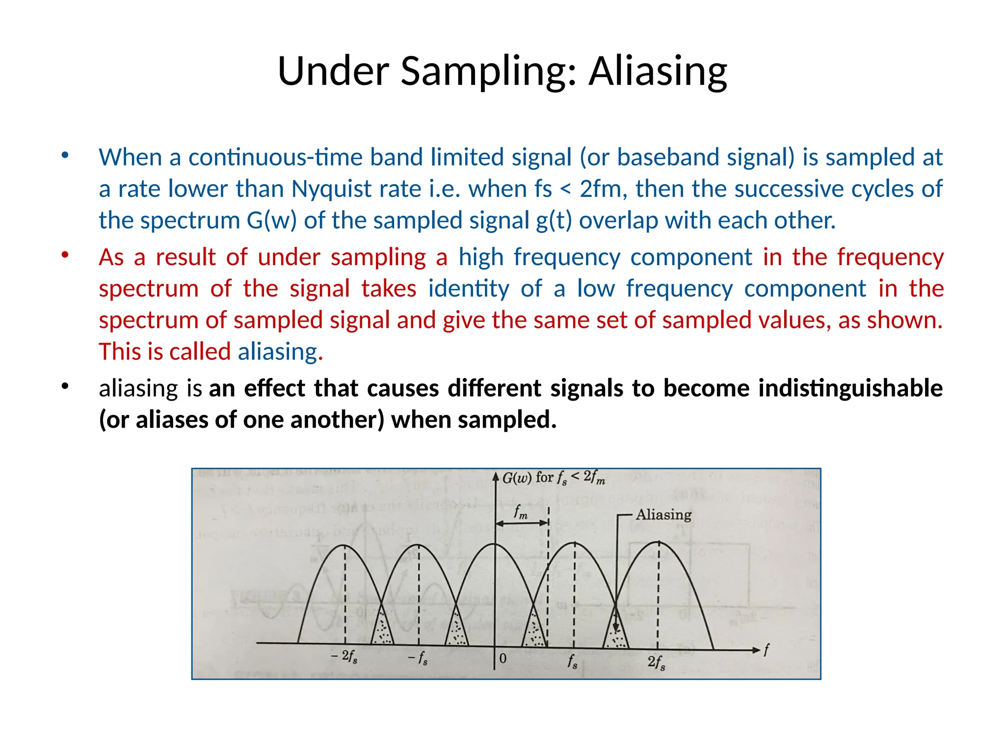
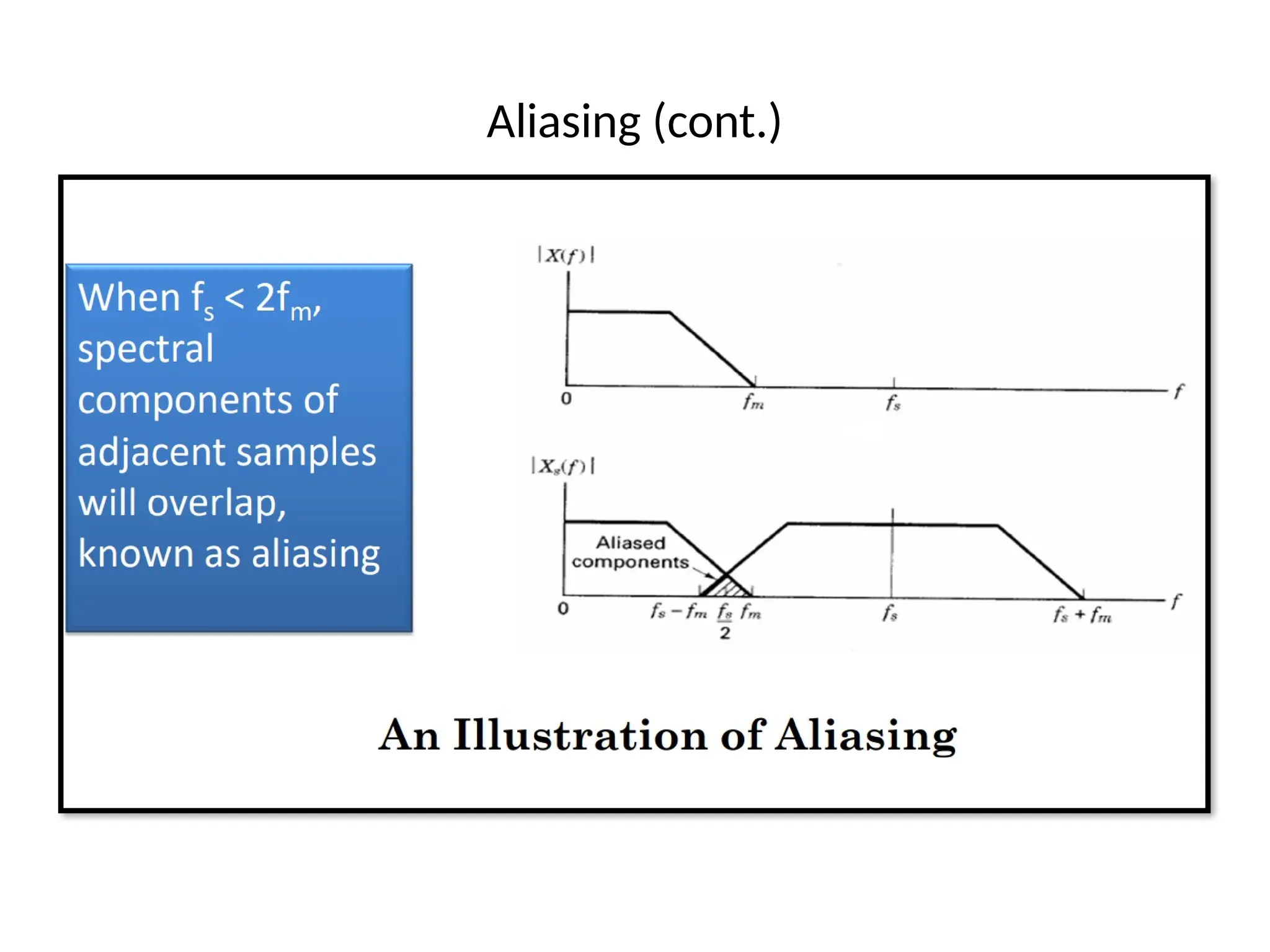
•When a continuous-time band limited signal (or baseband signal) is sampled at
a rate lower than Nyquist rate i.e. when fs < 2fm, then the successive cycles of
the spectrum G(w) of the sampled signal g(t) overlap with each other.
• As a result of under sampling a high frequency component in the frequency
spectrum of the signal takes identity of a low frequency component in the
spectrum of sampled signal and give the same set of sampled values, as shown.
This is called aliasing.
• aliasing is an effect that causes different signals to become indistinguishable
(or aliases of one another) when sampled.
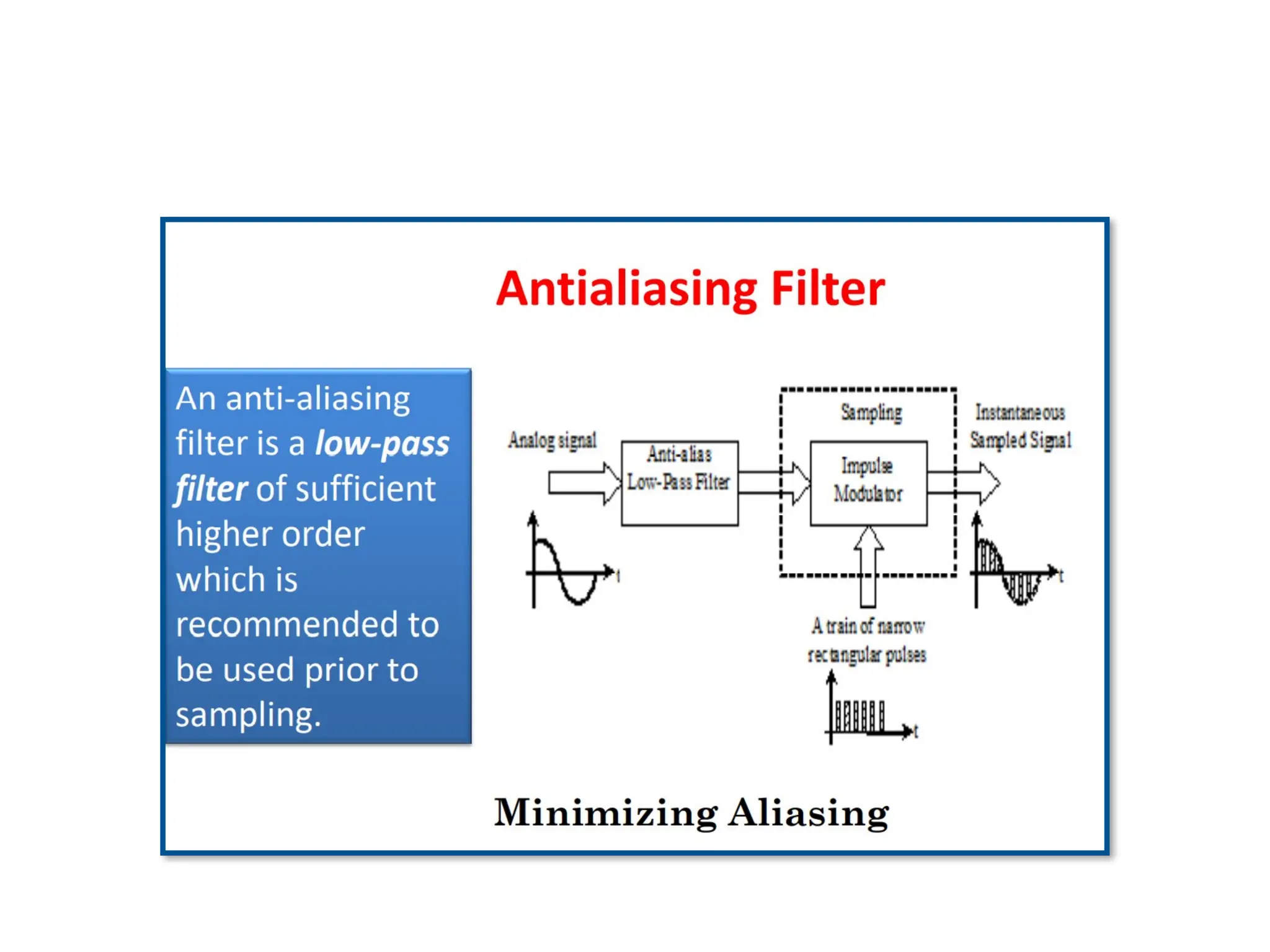
Solution: Anti-Aliasing AnalogFilter
• All physically realizable signals are not completely band
limited.
• If there is a significant amount of energy in frequencies above
half the sampling frequency (fs /2), aliasing will occur.
• Aliasing can be prevented by first passing the analog signal
through an anti aliasing filter also called a pre-filter, before
sampling is performed.
• The anti-aliasing filter is simply a LPF with cutoff frequency
equal to half the sample rate.
39.
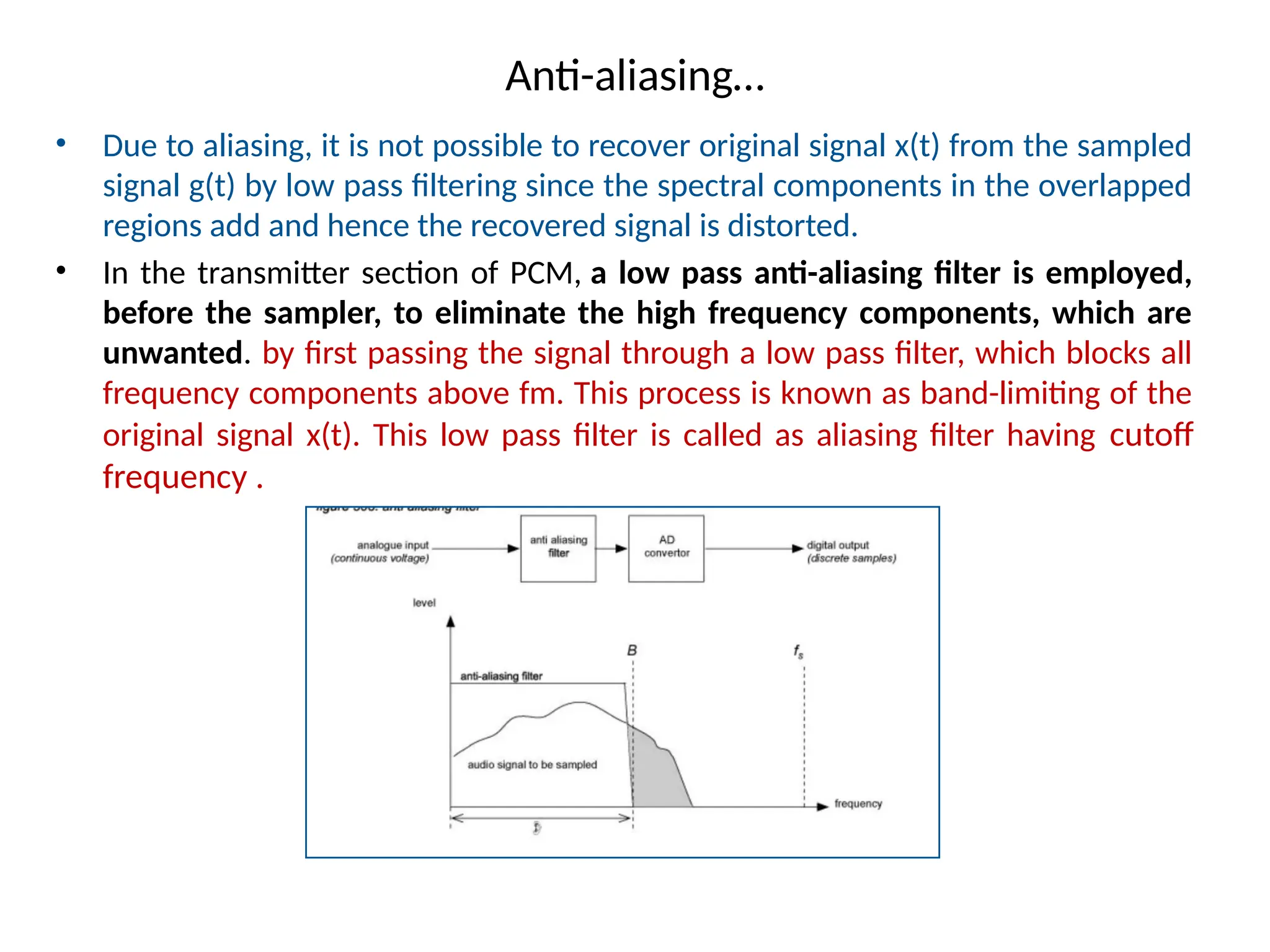
Anti-aliasing…
• Due toaliasing, it is not possible to recover original signal x(t) from the sampled
signal g(t) by low pass filtering since the spectral components in the overlapped
regions add and hence the recovered signal is distorted.
• In the transmitter section of PCM, a low pass anti-aliasing filter is employed,
before the sampler, to eliminate the high frequency components, which are
unwanted. by first passing the signal through a low pass filter, which blocks all
frequency components above fm. This process is known as band-limiting of the
original signal x(t). This low pass filter is called as aliasing filter having cutoff
frequency .
40.
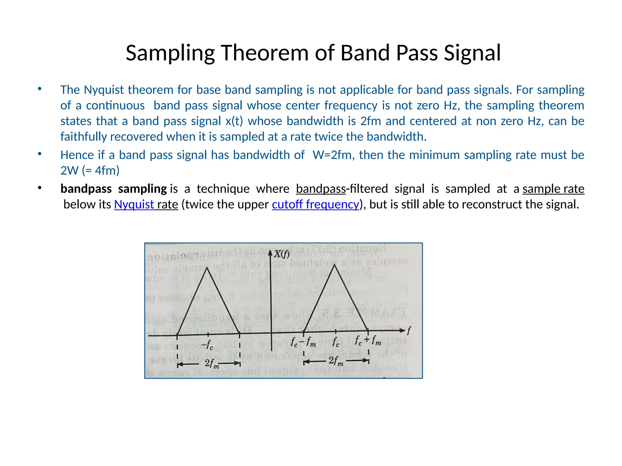
Sampling Theorem ofBand Pass Signal
• The Nyquist theorem for base band sampling is not applicable for band pass signals. For sampling
of a continuous band pass signal whose center frequency is not zero Hz, the sampling theorem
states that a band pass signal x(t) whose bandwidth is 2fm and centered at non zero Hz, can be
faithfully recovered when it is sampled at a rate twice the bandwidth.
• Hence if a band pass signal has bandwidth of W=2fm, then the minimum sampling rate must be
2W (= 4fm)
• bandpass sampling is a technique where bandpass-filtered signal is sampled at a sample rate
below its Nyquist rate (twice the upper cutoff frequency), but is still able to reconstruct the signal.
41.
Band pass Sampling:Advantages
• Band pass sampling requires less bandwidth to reconstruct the signal as compared to baseband sampling.
(fs)LPS = 2fm = Nyquist Sampling
• The sampling frequency of Bandpass signal (fs)BPF is less than the sampling frequency of a low pass filter (fs)LPS.
i.e. (fs)BPF < (fs)LPS
This implies that (Ts)BPS > (Ts)LPS
• Since the sampling interval is relatively large, this implies that the speed requirement is less.
• Because of less speed requirement, it will store less number of samples compared to low pass sampling. It
will, therefore, decrease the memory requirement because it stores fewer samples when compared to low-
pass sampling.
42.
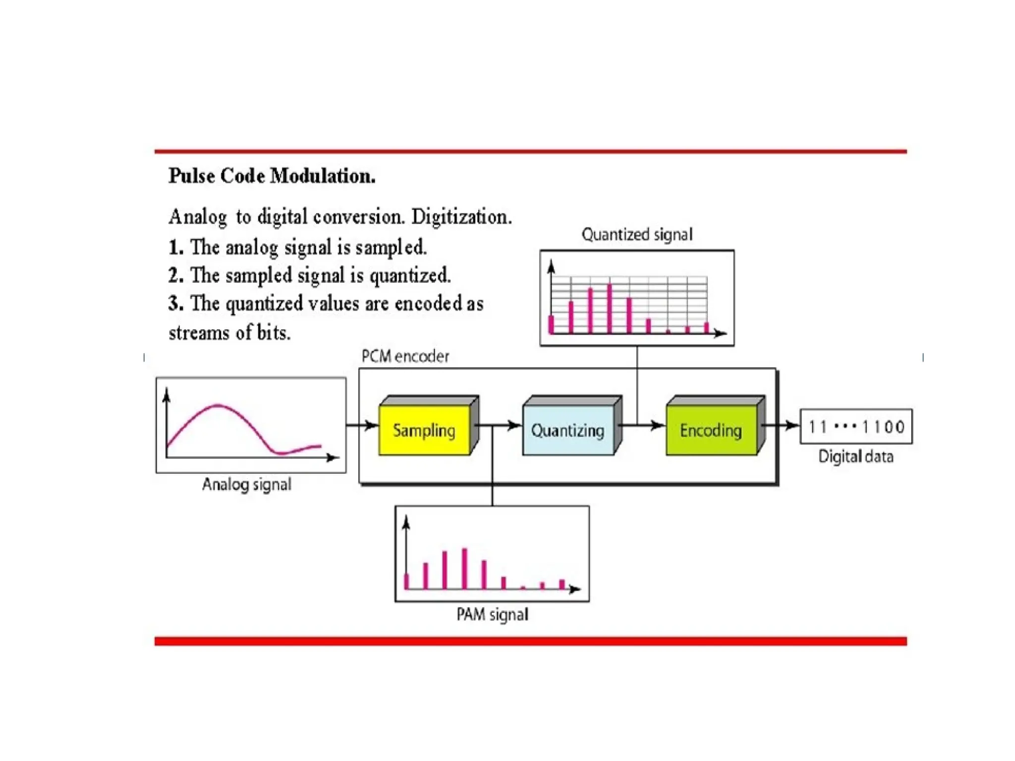
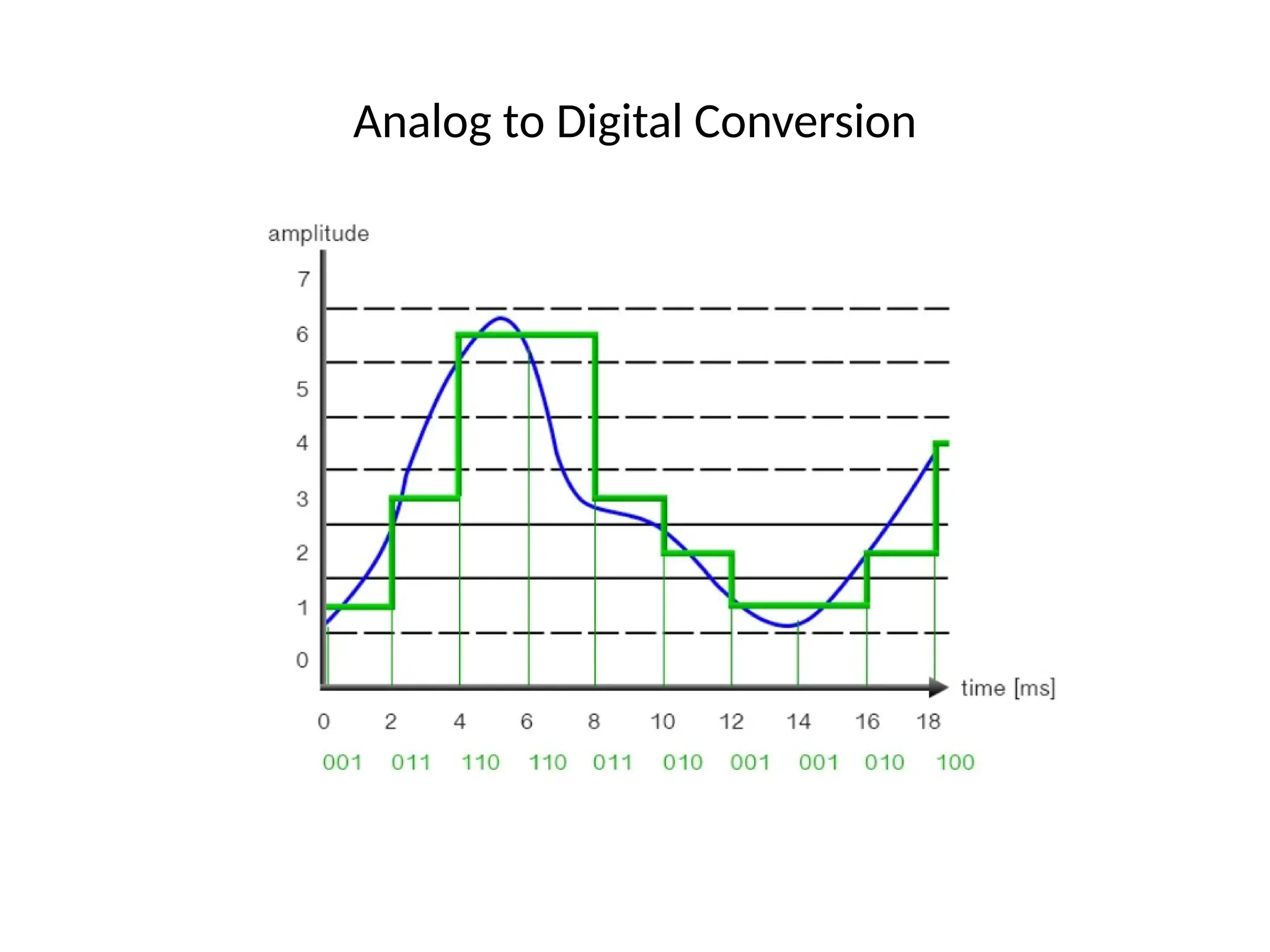
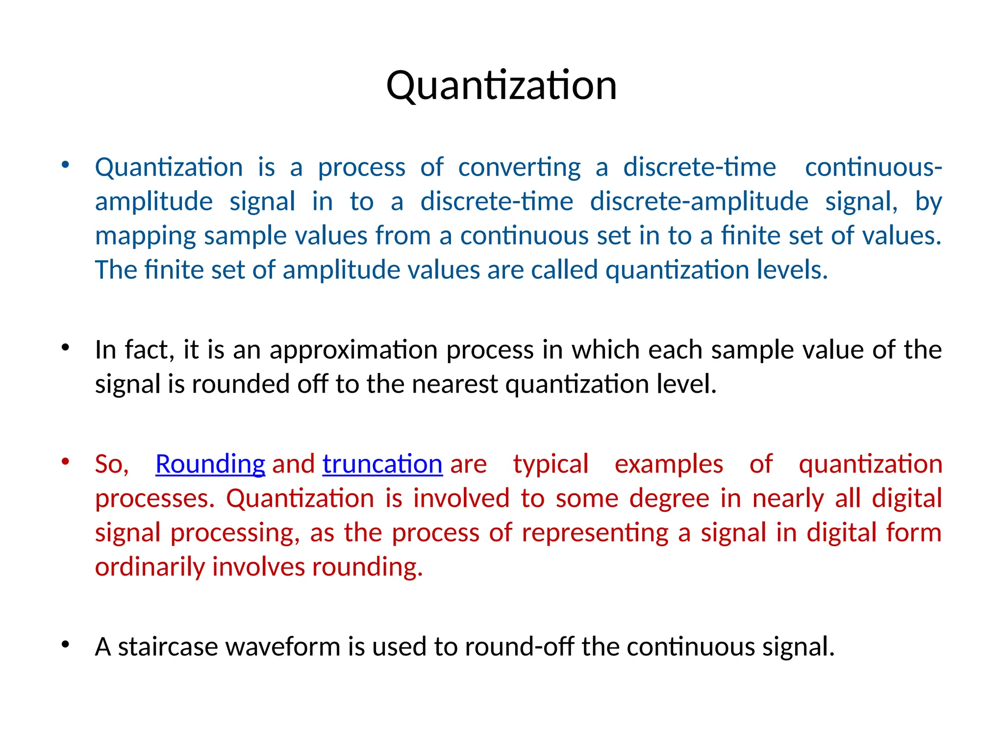
Quantization
• Quantization isa process of converting a discrete-time continuous-
amplitude signal in to a discrete-time discrete-amplitude signal, by
mapping sample values from a continuous set in to a finite set of values.
The finite set of amplitude values are called quantization levels.
• In fact, it is an approximation process in which each sample value of the
signal is rounded off to the nearest quantization level.
• So, Rounding and truncation are typical examples of quantization
processes. Quantization is involved to some degree in nearly all digital
signal processing, as the process of representing a signal in digital form
ordinarily involves rounding.
• A staircase waveform is used to round-off the continuous signal.
43.
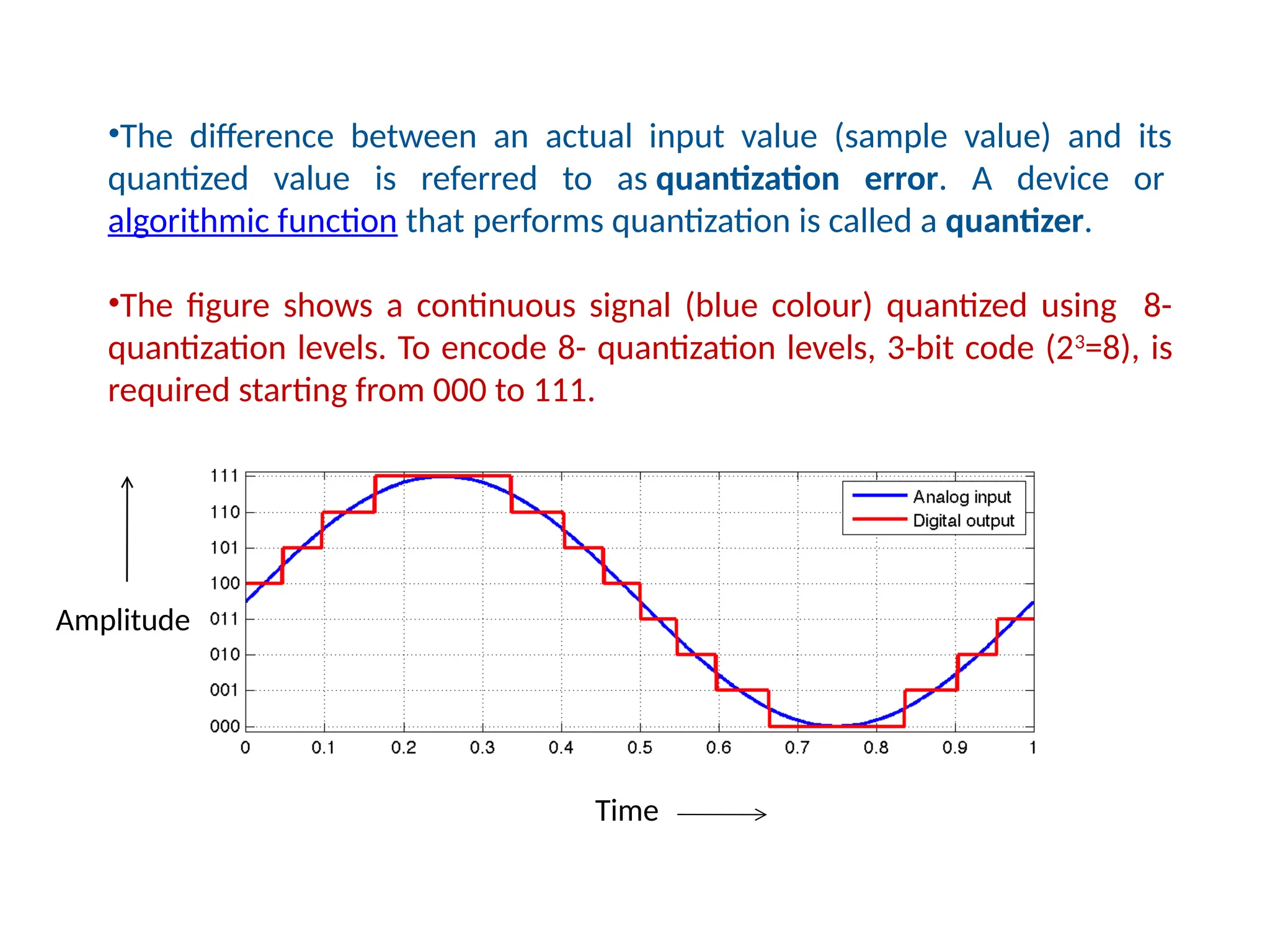
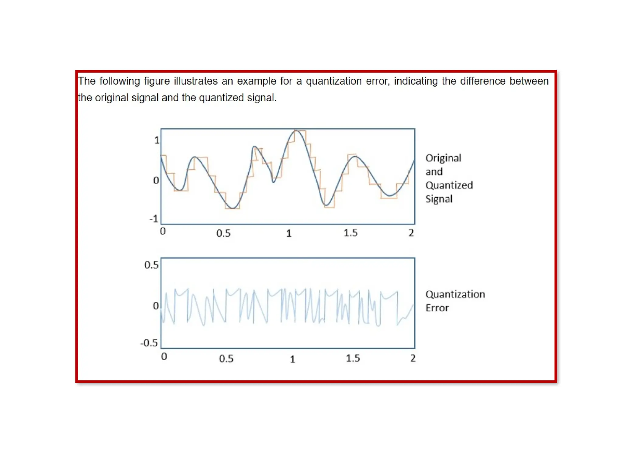
•The difference betweenan actual input value (sample value) and its
quantized value is referred to as quantization error. A device or
algorithmic function that performs quantization is called a quantizer.
•The figure shows a continuous signal (blue colour) quantized using 8-
quantization levels. To encode 8- quantization levels, 3-bit code (23
=8), is
required starting from 000 to 111.
Time
Amplitude
45.
Types of Quantization
Thereare two types of Quantization:
1. Uniform Quantization
2. Non-uniform Quantization.
• The type of quantization in which the quantization levels
are uniformly spaced is termed as a Uniform
Quantization.
• The type of quantization in which the quantization levels
are unequal and mostly the relation between them is
logarithmic, is termed as a Non-uniform Quantization.
46.
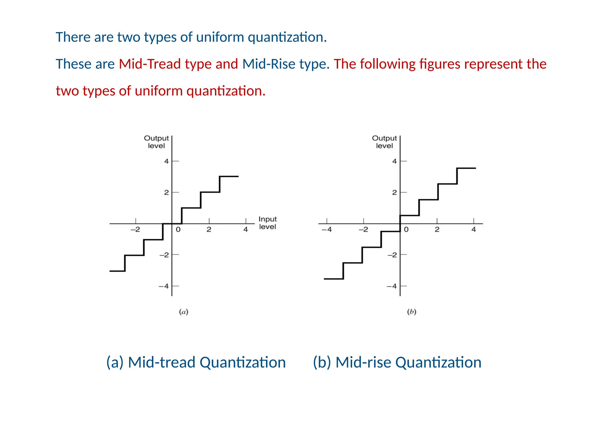
(a) Mid-tread Quantization(b) Mid-rise Quantization
There are two types of uniform quantization.
These are Mid-Tread type and Mid-Rise type. The following figures represent the
two types of uniform quantization.
47.
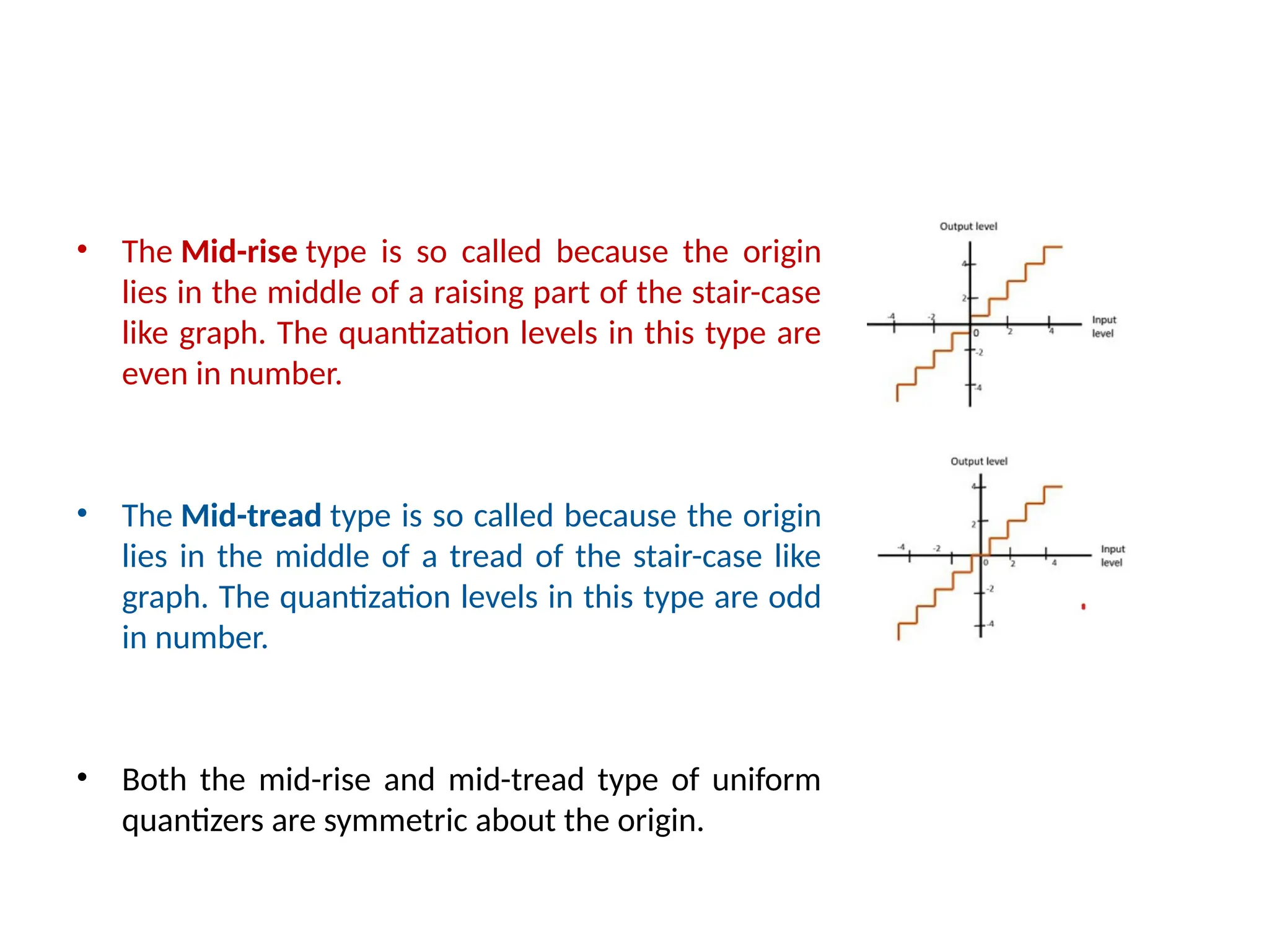
• The Mid-risetype is so called because the origin
lies in the middle of a raising part of the stair-case
like graph. The quantization levels in this type are
even in number.
• The Mid-tread type is so called because the origin
lies in the middle of a tread of the stair-case like
graph. The quantization levels in this type are odd
in number.
• Both the mid-rise and mid-tread type of uniform
quantizers are symmetric about the origin.
48.
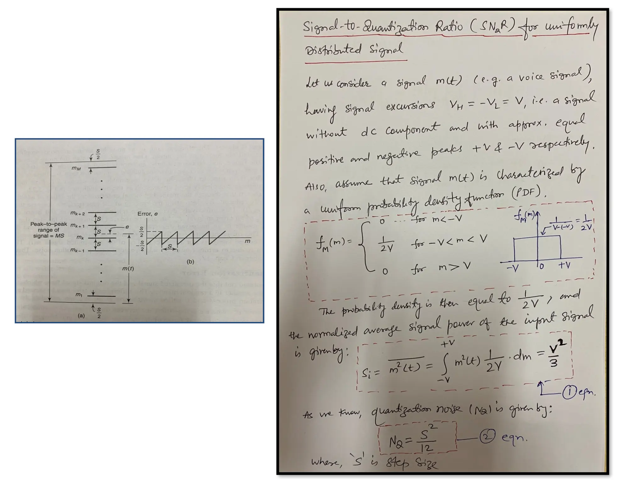
Step Size &Quantization Error
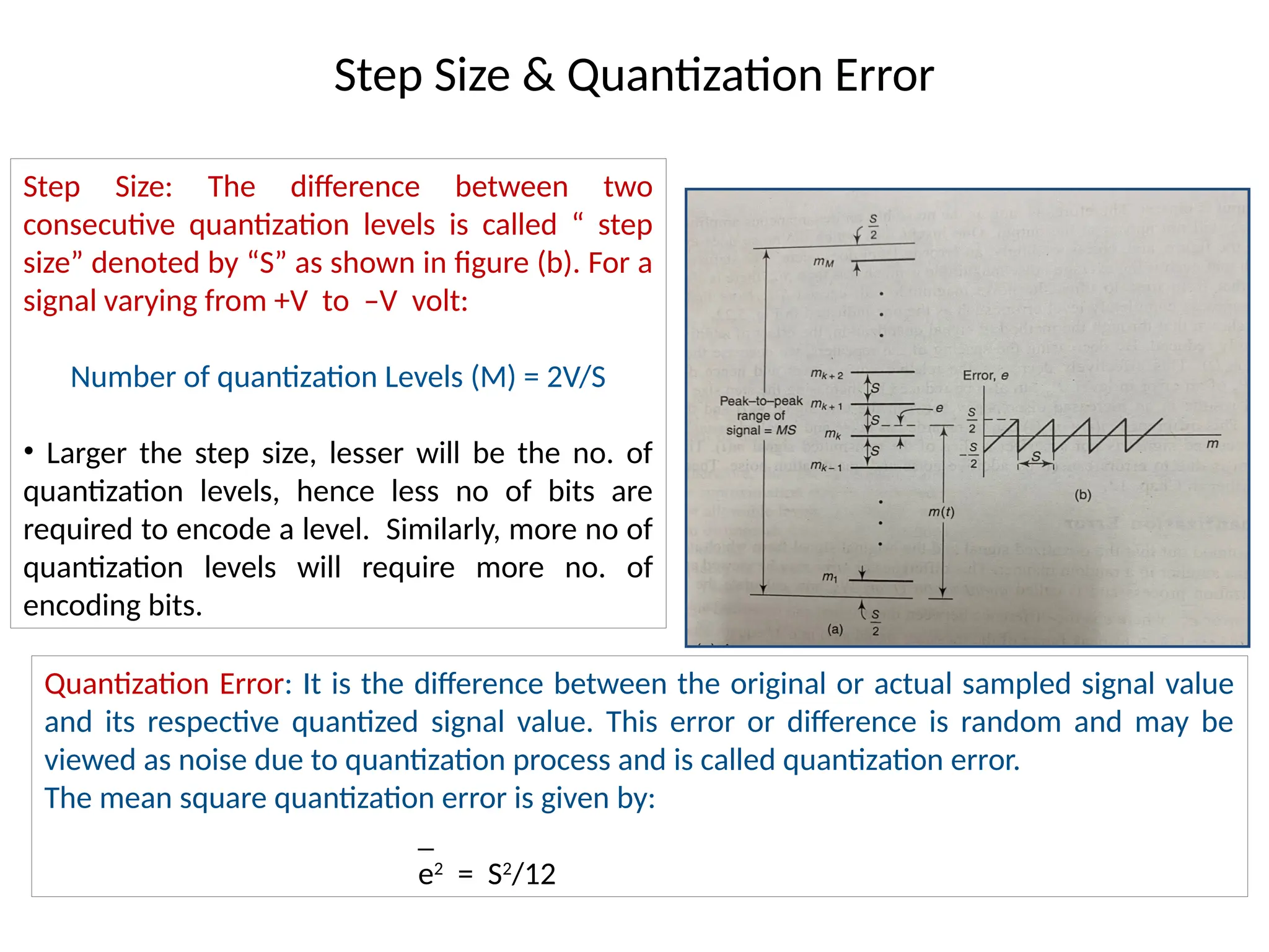
Step Size: The difference between two
consecutive quantization levels is called “ step
size” denoted by “S” as shown in figure (b). For a
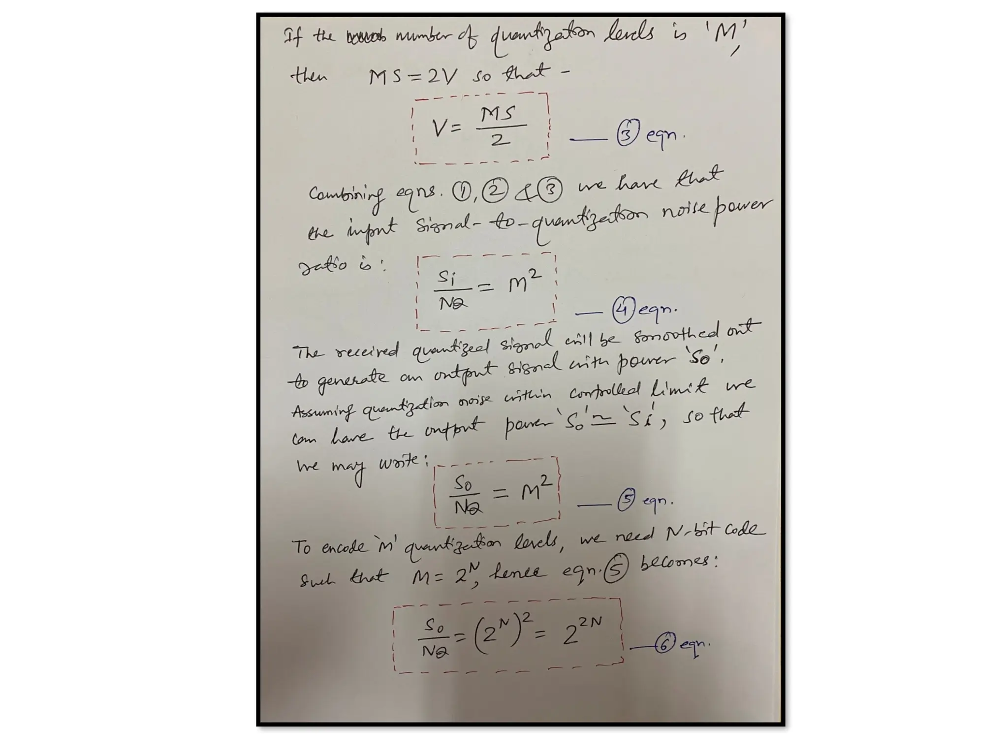
signal varying from +V to –V volt:
Number of quantization Levels (M) = 2V/S
• Larger the step size, lesser will be the no. of
quantization levels, hence less no of bits are
required to encode a level. Similarly, more no of
quantization levels will require more no. of
encoding bits.
Quantization Error: It is the difference between the original or actual sampled signal value
and its respective quantized signal value. This error or difference is random and may be
viewed as noise due to quantization process and is called quantization error.
The mean square quantization error is given by:
_
e2
= S2
/12
49.
Example: Quantization andencoding of a continuous signal with excursions from -4
Volt to +4 Volt
Step Size =[4-(-4)]/8 = 1 Volt
Eight quantization levels can
be located at :
-3.5, -2.5……+2.5, +3.5 Volt.
50.
Non-uniform Quantization: Companding
•In uniform quantization, the step size is kept fixed (constant) irrespective
of the signal level. As a result, quantization of weak signals produces high
quantization error/noise as compared to quantization error of stronger
signals.
• For example: in speech communication, the range of voltages covered by
speech signals, from the peaks of loud talk to the weak passages of weak
talk, is on the order of 1000 to 1. From practical point of view it is always
desirable to keep Signal-to-quantization Noise ratio to remain essentially
constant for such a wide dynamic range of input power levels.
• Otherwise, it causes lower values of SNR for weak signals, thus the
recovery of weak signals at receiving end is erroneous (digital signals) or
distorted (analog signals).
• In order to overcome this problem, robust quantization is required known
as non-uniform quantization, which is characterized by a step size that
increases as the separation from the origin of the transfer characteristics is
increased.
51.
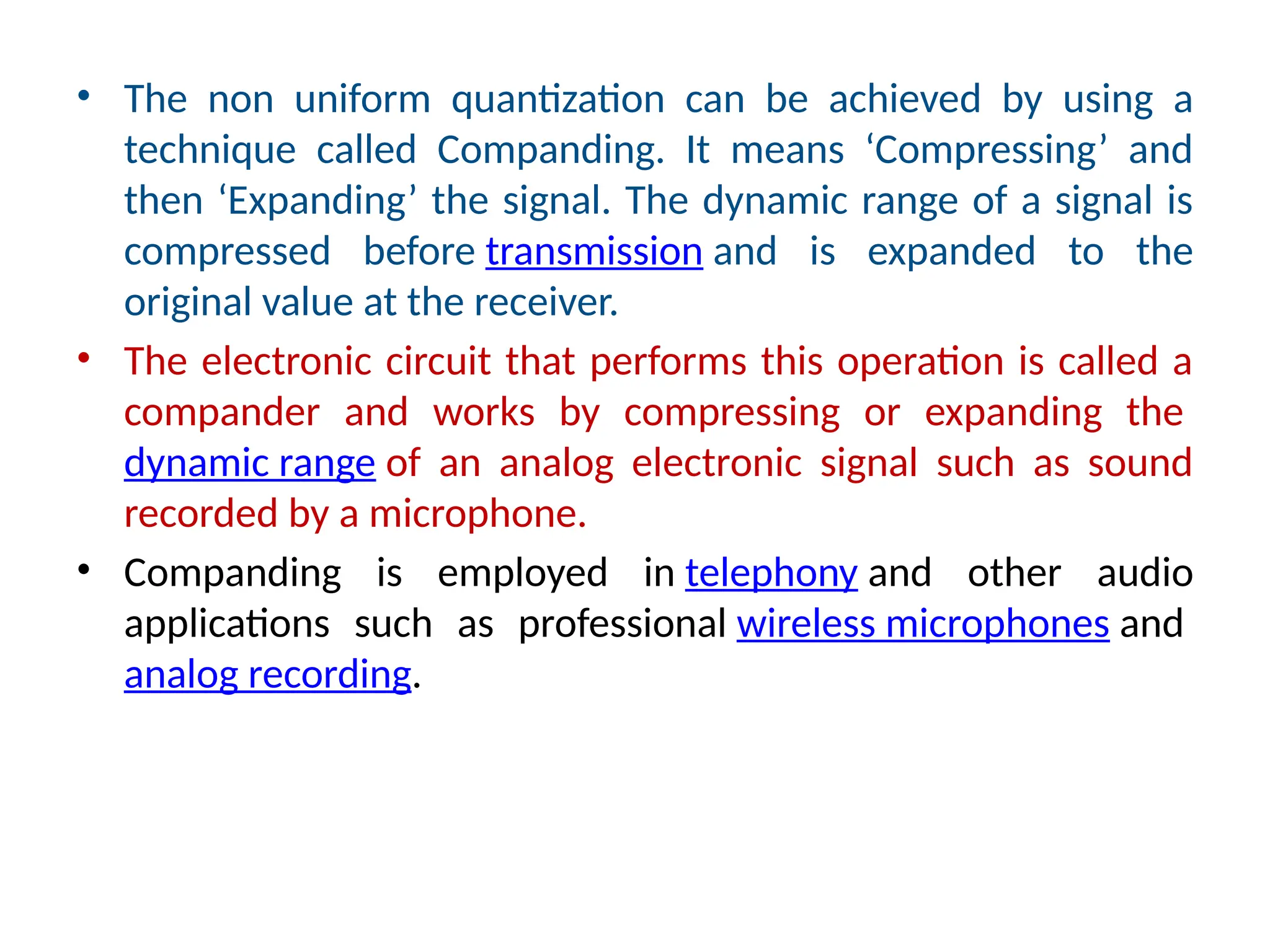
• The nonuniform quantization can be achieved by using a
technique called Companding. It means ‘Compressing’ and
then ‘Expanding’ the signal. The dynamic range of a signal is
compressed before transmission and is expanded to the
original value at the receiver.
• The electronic circuit that performs this operation is called a
compander and works by compressing or expanding the
dynamic range of an analog electronic signal such as sound
recorded by a microphone.
• Companding is employed in telephony and other audio
applications such as professional wireless microphones and
analog recording.
52.
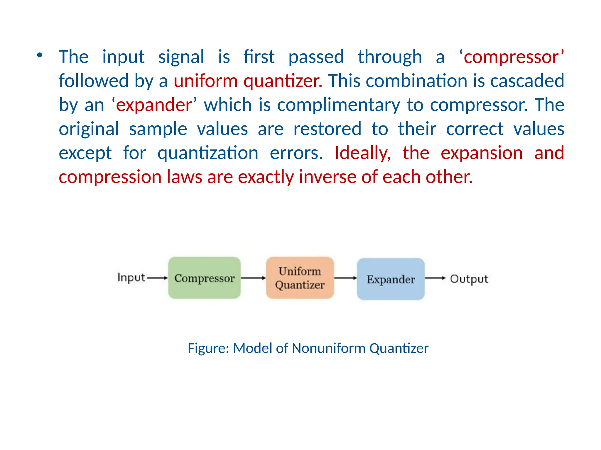
• The inputsignal is first passed through a ‘compressor’
followed by a uniform quantizer. This combination is cascaded
by an ‘expander’ which is complimentary to compressor. The
original sample values are restored to their correct values
except for quantization errors. Ideally, the expansion and
compression laws are exactly inverse of each other.
Figure: Model of Nonuniform Quantizer
53.
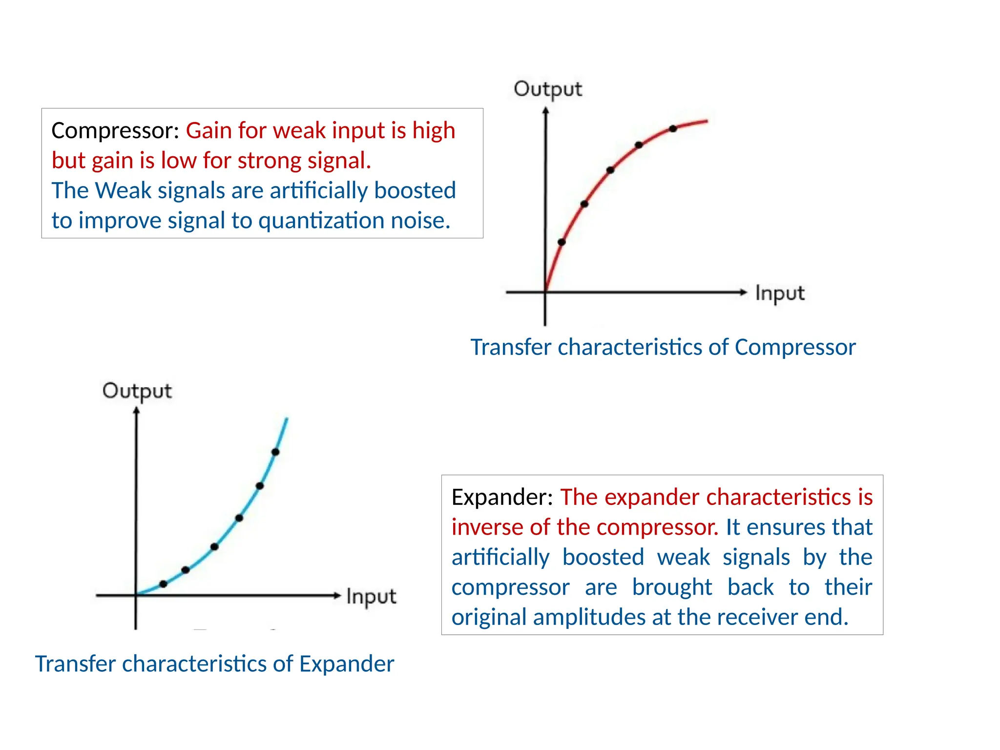
Transfer characteristics ofCompressor
Transfer characteristics of Expander
Compressor: Gain for weak input is high
but gain is low for strong signal.
The Weak signals are artificially boosted
to improve signal to quantization noise.
Expander: The expander characteristics is
inverse of the compressor. It ensures that
artificially boosted weak signals by the
compressor are brought back to their
original amplitudes at the receiver end.
54.
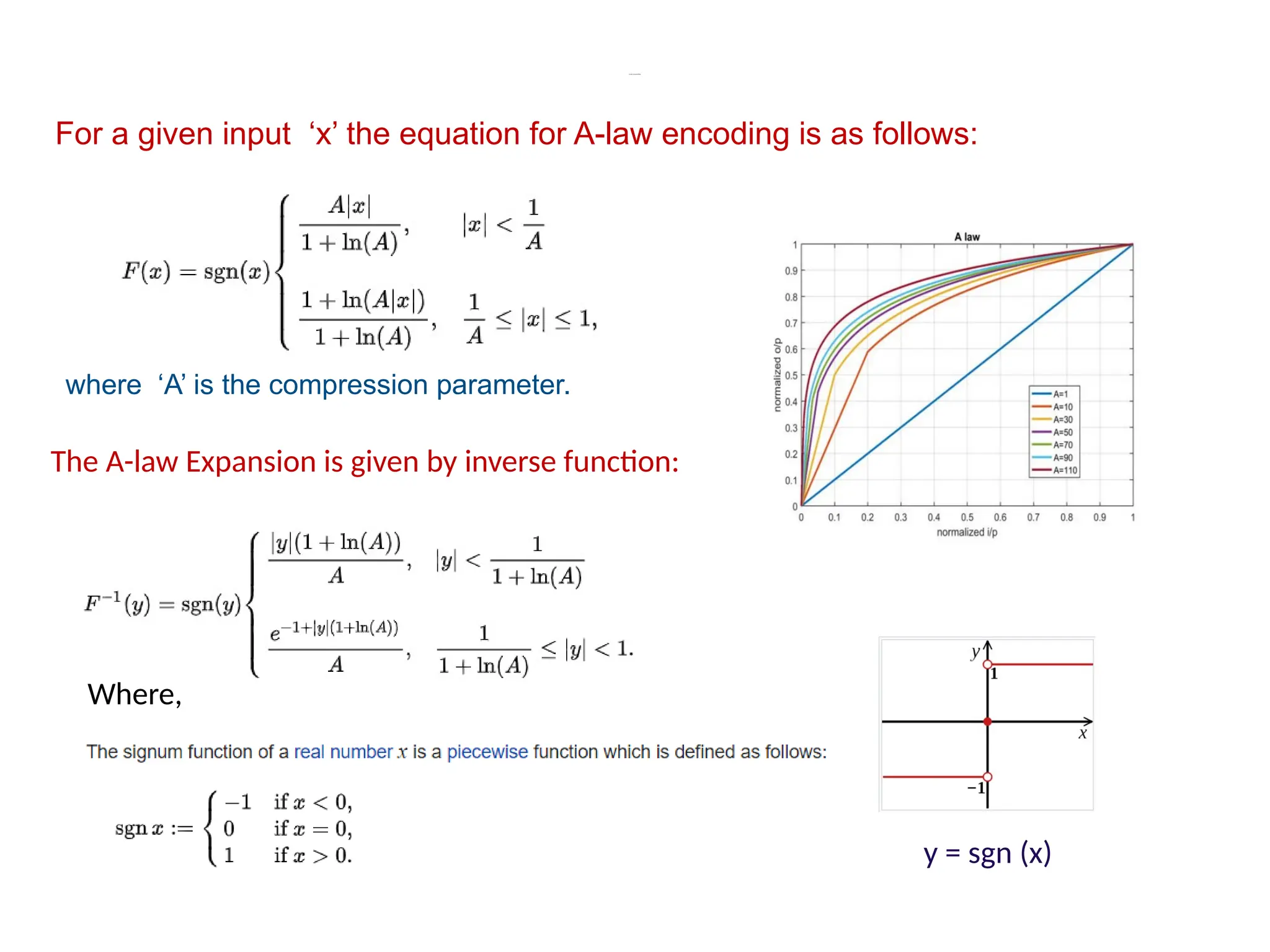
A-law Companding
For agiven input ‘x’ the equation for A-law encoding is as follows:
where ‘A’ is the compression parameter.
The A-law Expansion is given by inverse function:
Where,
y = sgn (x)
55.
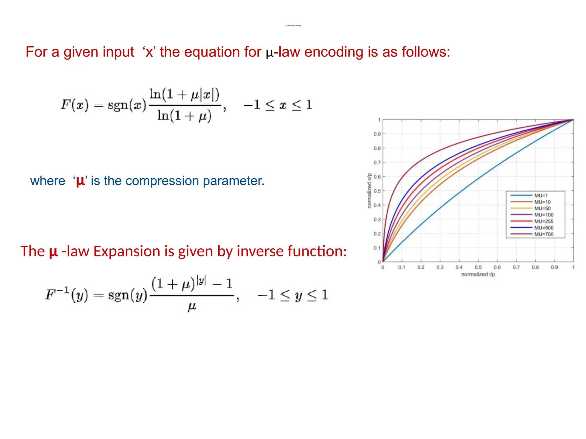
µ-law Companding
For agiven input ‘x’ the equation for µ-law encoding is as follows:
where ‘µ’ is the compression parameter.
The µ -law Expansion is given by inverse function:
56.
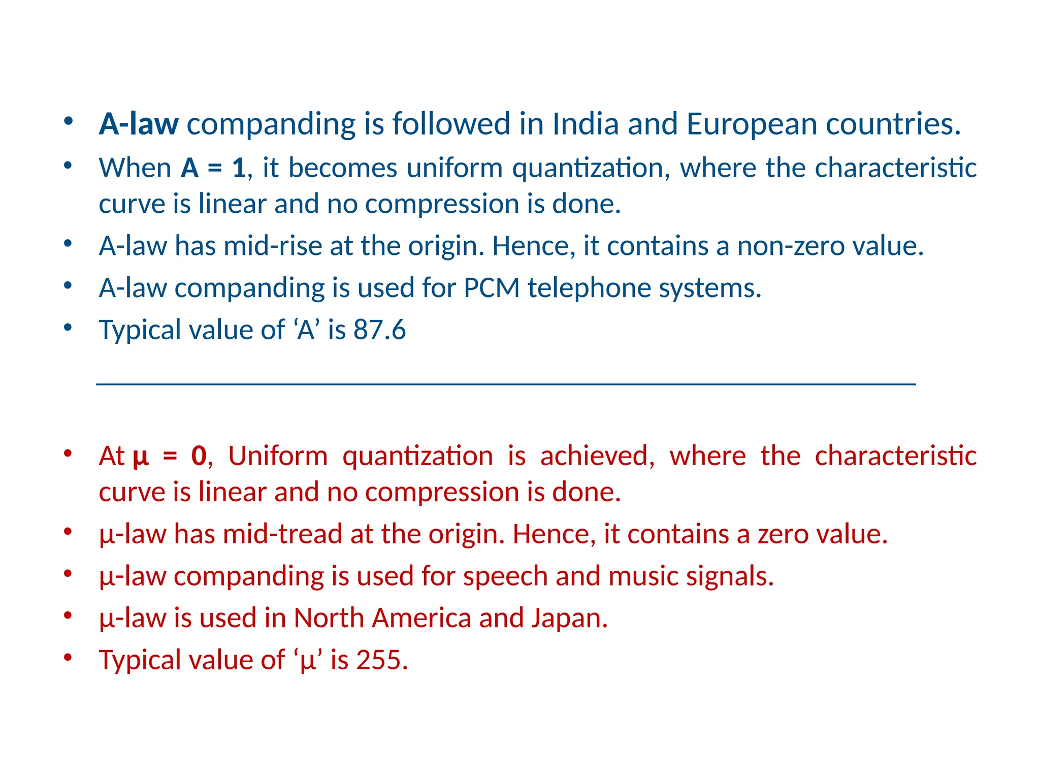
• A-law compandingis followed in India and European countries.
• When A = 1, it becomes uniform quantization, where the characteristic
curve is linear and no compression is done.
• A-law has mid-rise at the origin. Hence, it contains a non-zero value.
• A-law companding is used for PCM telephone systems.
• Typical value of ‘A’ is 87.6
_______________________________________________________
• At µ = 0, Uniform quantization is achieved, where the characteristic
curve is linear and no compression is done.
• µ-law has mid-tread at the origin. Hence, it contains a zero value.
• µ-law companding is used for speech and music signals.
• µ-law is used in North America and Japan.
• Typical value of ‘µ’ is 255.
57.
Applications of Companding
•Companding is used in digital telephony systems, compressing before input to an
analog-to-digital converter, and then expanding after a digital-to-analog converter.
• This is equivalent to using a non-linear ADC as in a T-carrier telephone system that
implements A-law or μ-law companding. This method is also used in digital file
formats for better SNR at lower bit depths.
• Professional wireless microphones do this since the dynamic range of the
microphone audio signal itself is larger than the dynamic range provided by radio
transmission. Companding also reduces the noise and crosstalk levels at the
receiver. Companders are used in concert audio systems and in some
noise reduction schemes.
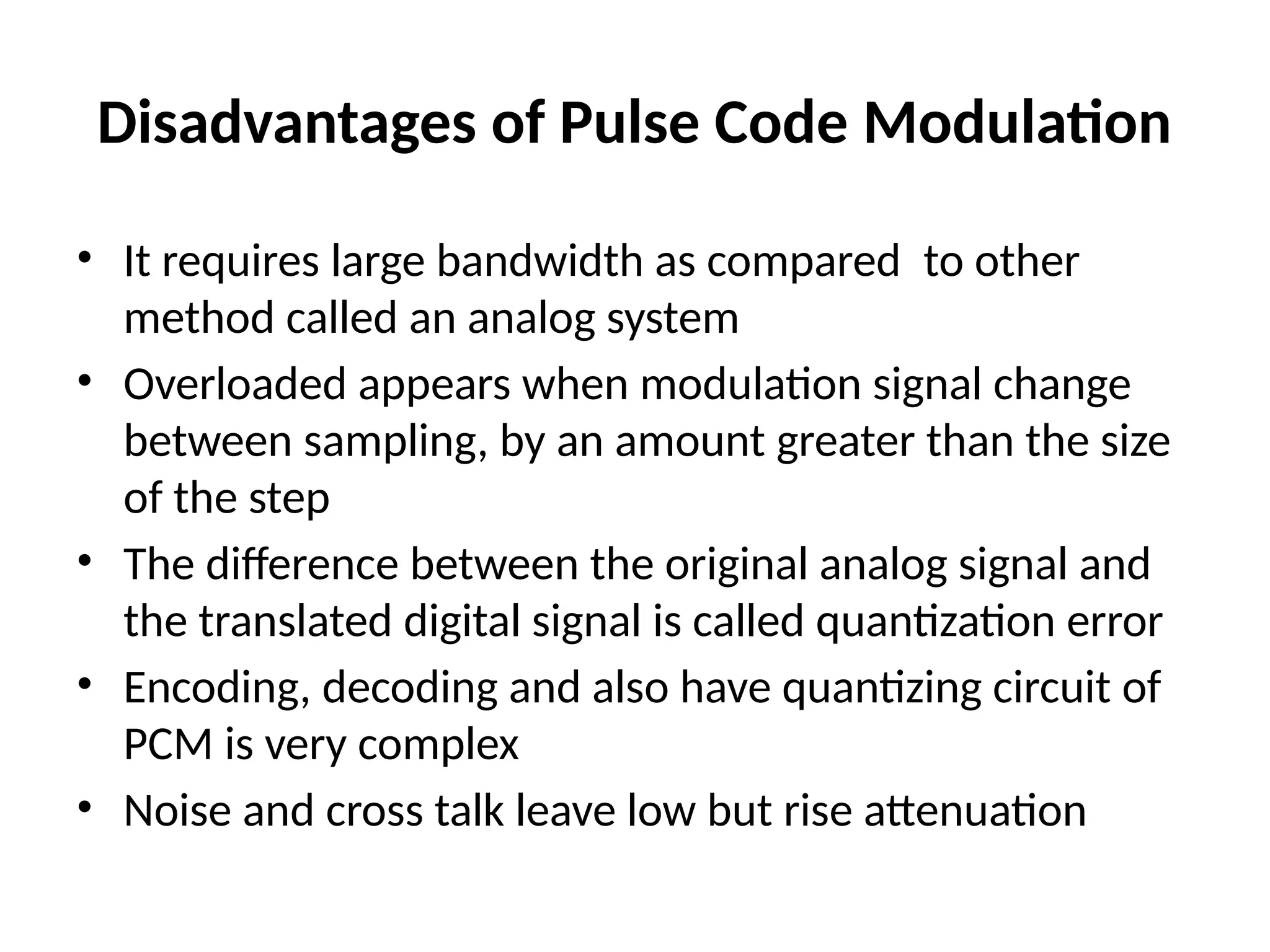
Disadvantages of PulseCode Modulation
• It requires large bandwidth as compared to other
method called an analog system
• Overloaded appears when modulation signal change
between sampling, by an amount greater than the size
of the step
• The difference between the original analog signal and
the translated digital signal is called quantization error
• Encoding, decoding and also have quantizing circuit of
PCM is very complex
• Noise and cross talk leave low but rise attenuation
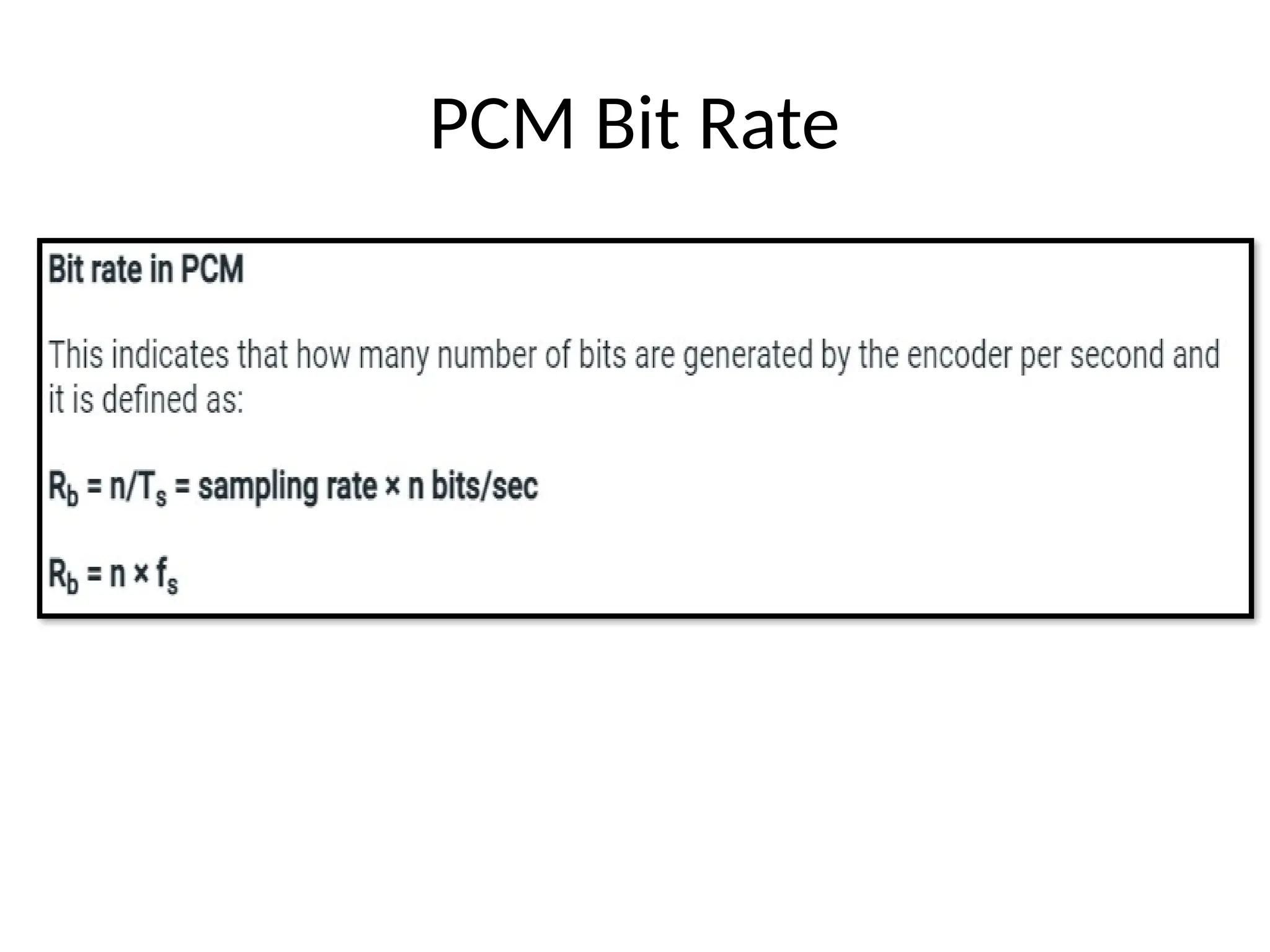
PCM Bandwidth
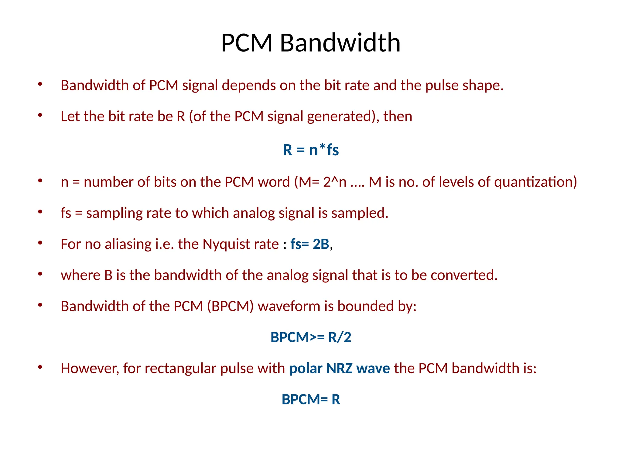
• Bandwidthof PCM signal depends on the bit rate and the pulse shape.
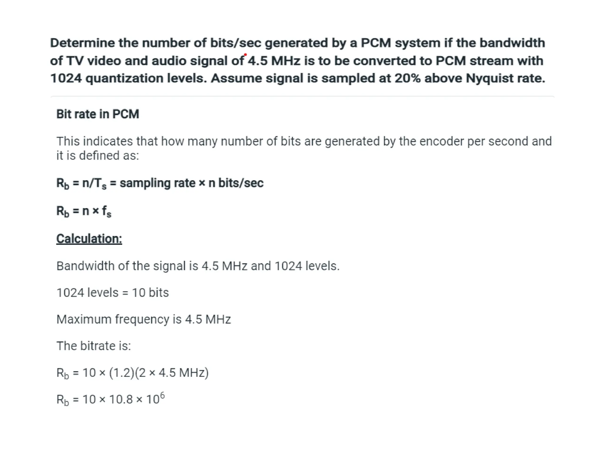
• Let the bit rate be R (of the PCM signal generated), then
R = n*fs
• n = number of bits on the PCM word (M= 2^n …. M is no. of levels of quantization)
• fs = sampling rate to which analog signal is sampled.
• For no aliasing i.e. the Nyquist rate : fs= 2B,
• where B is the bandwidth of the analog signal that is to be converted.
• Bandwidth of the PCM (BPCM) waveform is bounded by:
BPCM>= R/2
• However, for rectangular pulse with polar NRZ wave the PCM bandwidth is:
BPCM= R
70.
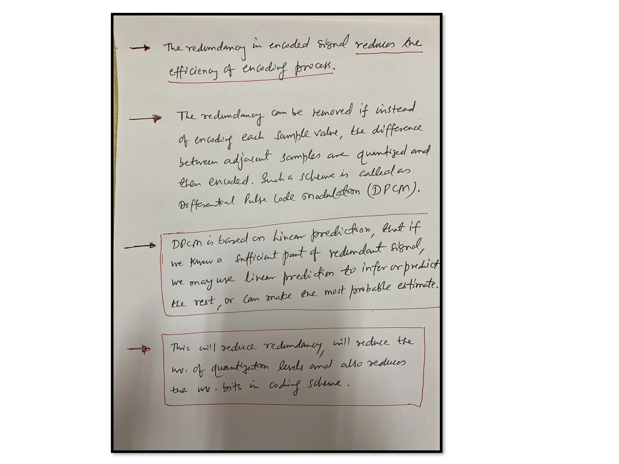
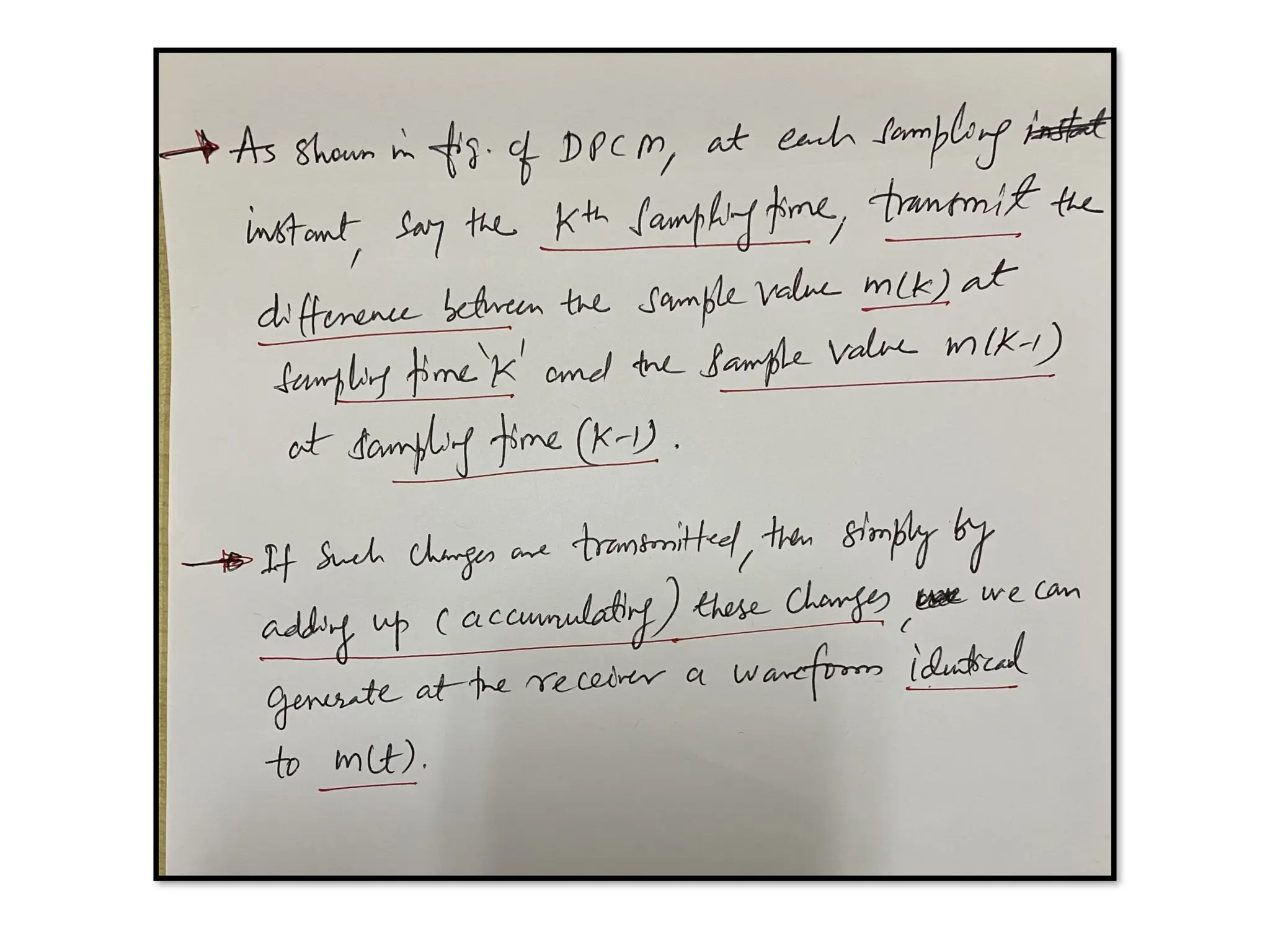
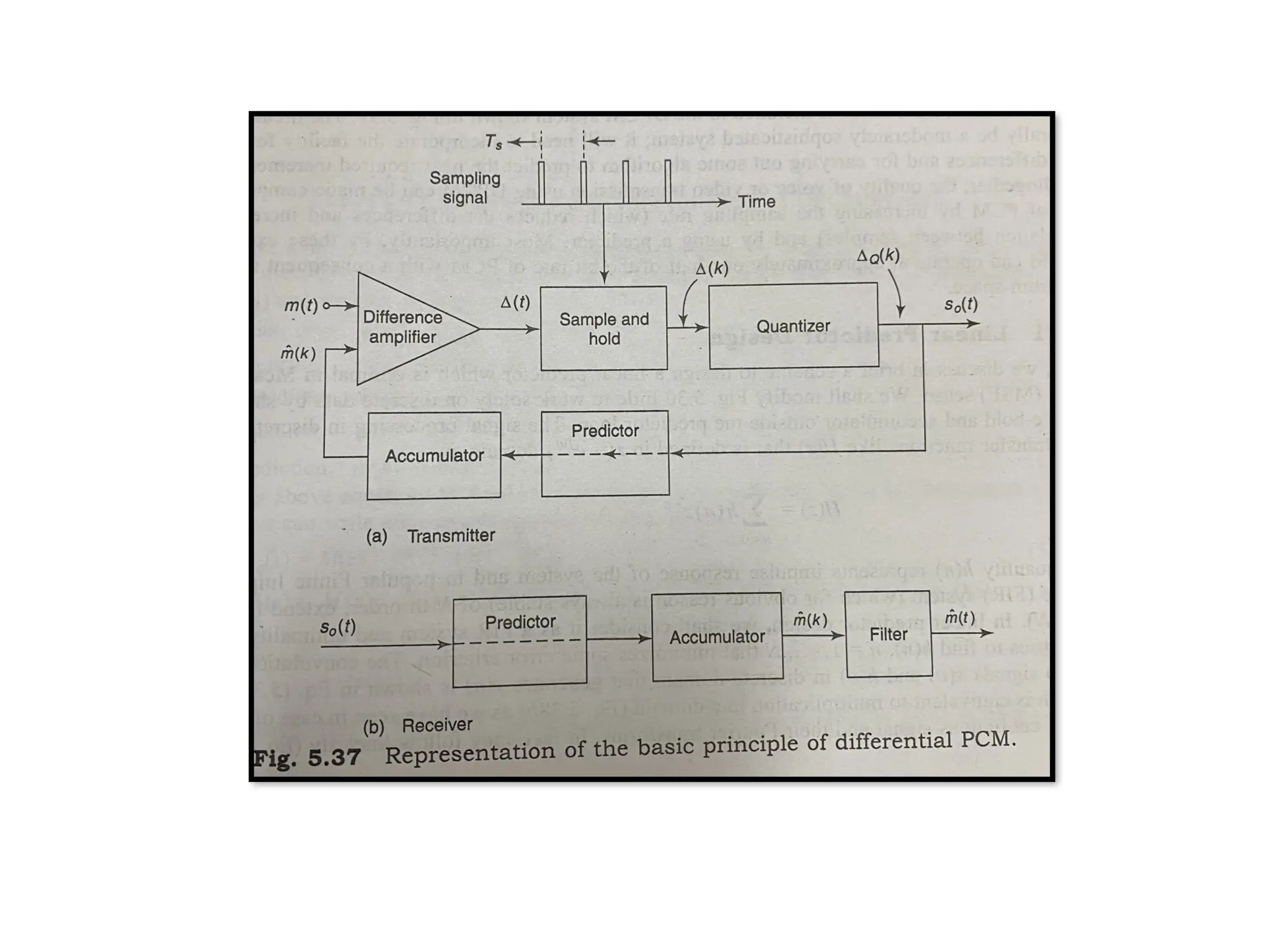
• ADVANTAGES OFDPCM:
1)BANDWIDTH REQUIREMENT OF DPCM IS LESS
COMPARED TO PCM.
2) QUANTIZATION ERROR IS REDUCED BECAUSE
OF PREDICTION FILTER.
3) NUMBERS OF BITS USED TO REPRESENT ONE
SAMPLE VALUE ARE ALSO REDUCED
COMPARED TO PCM.
71.
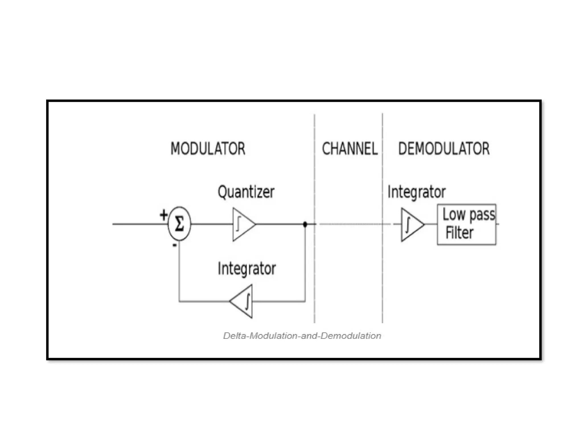
Delta Modulation (DM)
•A delta modulation is a DPCM scheme in which the difference
signal Δ(t) is encoded into just a single bit, hence
delta Modulator is called as a single bit modulator.
• It comprises a 1-bit quantizer and a delay circuit along with two
summer circuits.
• DM is the simplest form of differential pulse-code modulation
(DPCM) where the difference between successive samples is
encoded into n-bit data streams. In delta modulation, the
transmitted data are reduced to a 1-bit data stream.
• Only the change of information is sent, that is, only an increase
or decrease of the signal amplitude from the previous sample is
sent whereas a no-change condition causes the modulated
signal to remain at the same 0 or 1 state of the previous
sample.
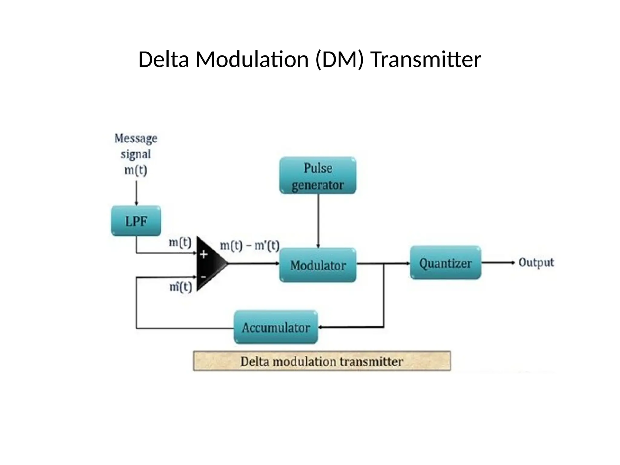
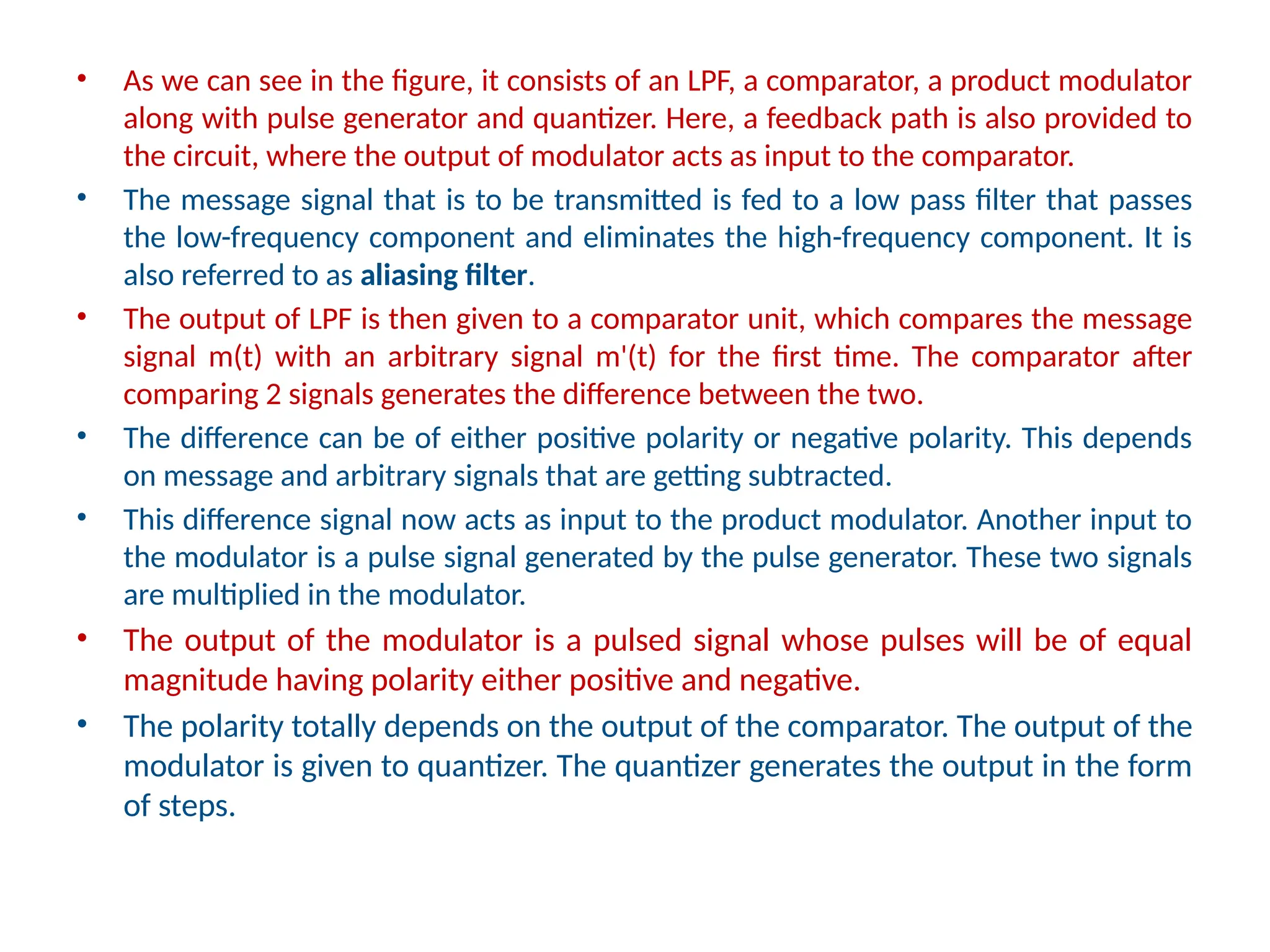
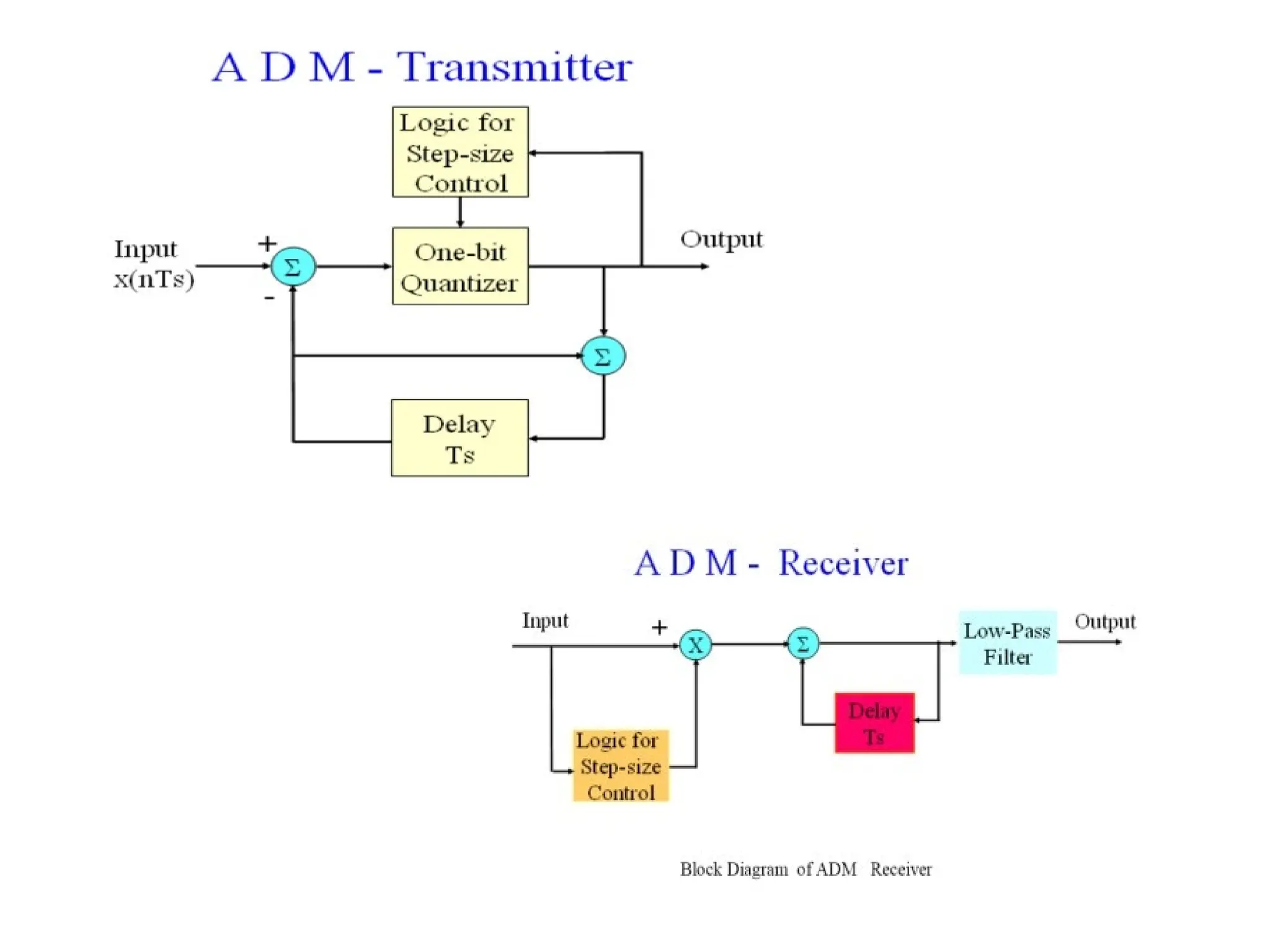
• As wecan see in the figure, it consists of an LPF, a comparator, a product modulator
along with pulse generator and quantizer. Here, a feedback path is also provided to
the circuit, where the output of modulator acts as input to the comparator.
• The message signal that is to be transmitted is fed to a low pass filter that passes
the low-frequency component and eliminates the high-frequency component. It is
also referred to as aliasing filter.
• The output of LPF is then given to a comparator unit, which compares the message
signal m(t) with an arbitrary signal m'(t) for the first time. The comparator after
comparing 2 signals generates the difference between the two.
• The difference can be of either positive polarity or negative polarity. This depends
on message and arbitrary signals that are getting subtracted.
• This difference signal now acts as input to the product modulator. Another input to
the modulator is a pulse signal generated by the pulse generator. These two signals
are multiplied in the modulator.
• The output of the modulator is a pulsed signal whose pulses will be of equal
magnitude having polarity either positive and negative.
• The polarity totally depends on the output of the comparator. The output of the
modulator is given to quantizer. The quantizer generates the output in the form
of steps.
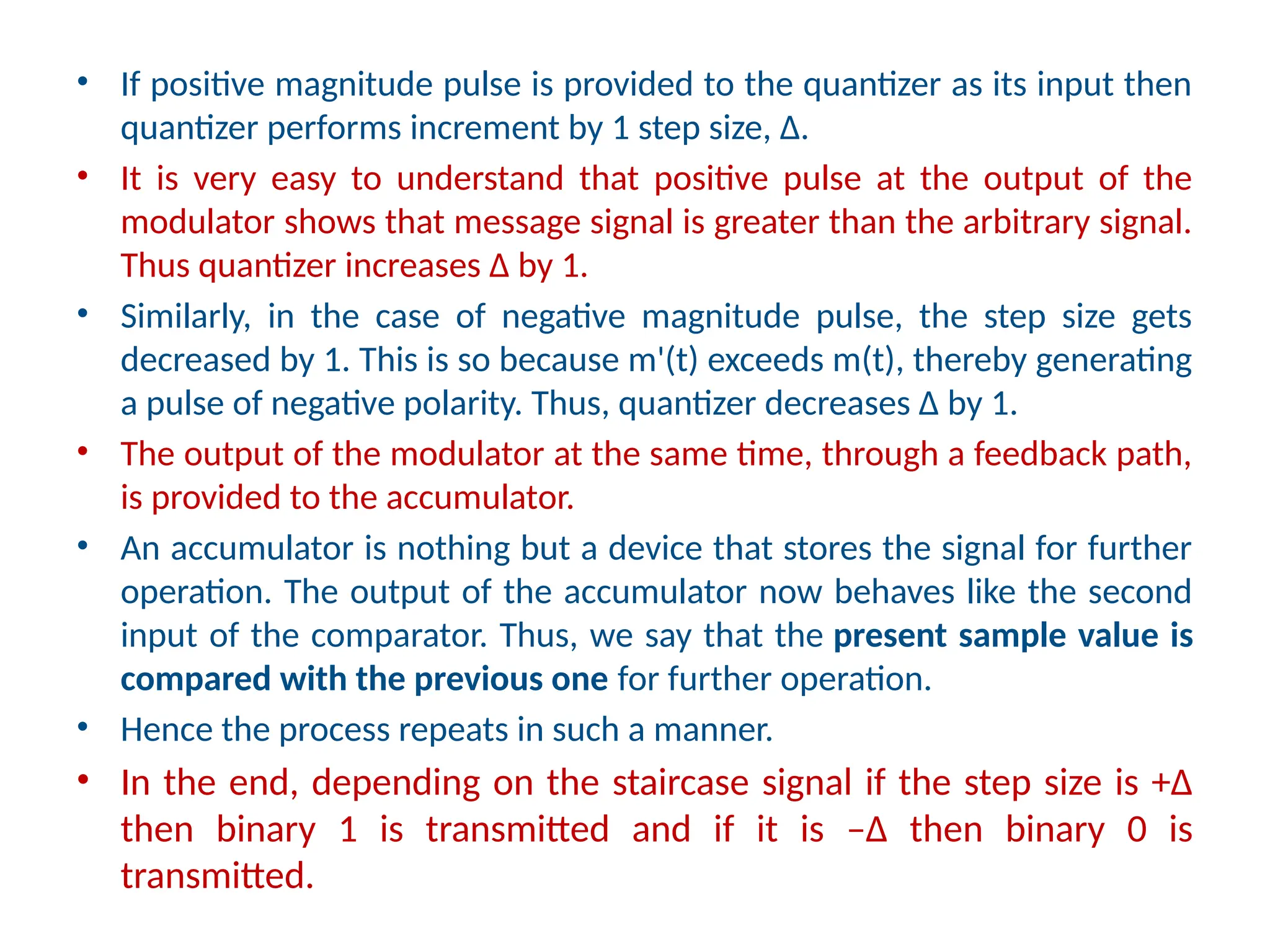
75.
• If positivemagnitude pulse is provided to the quantizer as its input then
quantizer performs increment by 1 step size, Δ.
• It is very easy to understand that positive pulse at the output of the
modulator shows that message signal is greater than the arbitrary signal.
Thus quantizer increases Δ by 1.
• Similarly, in the case of negative magnitude pulse, the step size gets
decreased by 1. This is so because m'(t) exceeds m(t), thereby generating
a pulse of negative polarity. Thus, quantizer decreases Δ by 1.
• The output of the modulator at the same time, through a feedback path,
is provided to the accumulator.
• An accumulator is nothing but a device that stores the signal for further
operation. The output of the accumulator now behaves like the second
input of the comparator. Thus, we say that the present sample value is
compared with the previous one for further operation.
• Hence the process repeats in such a manner.
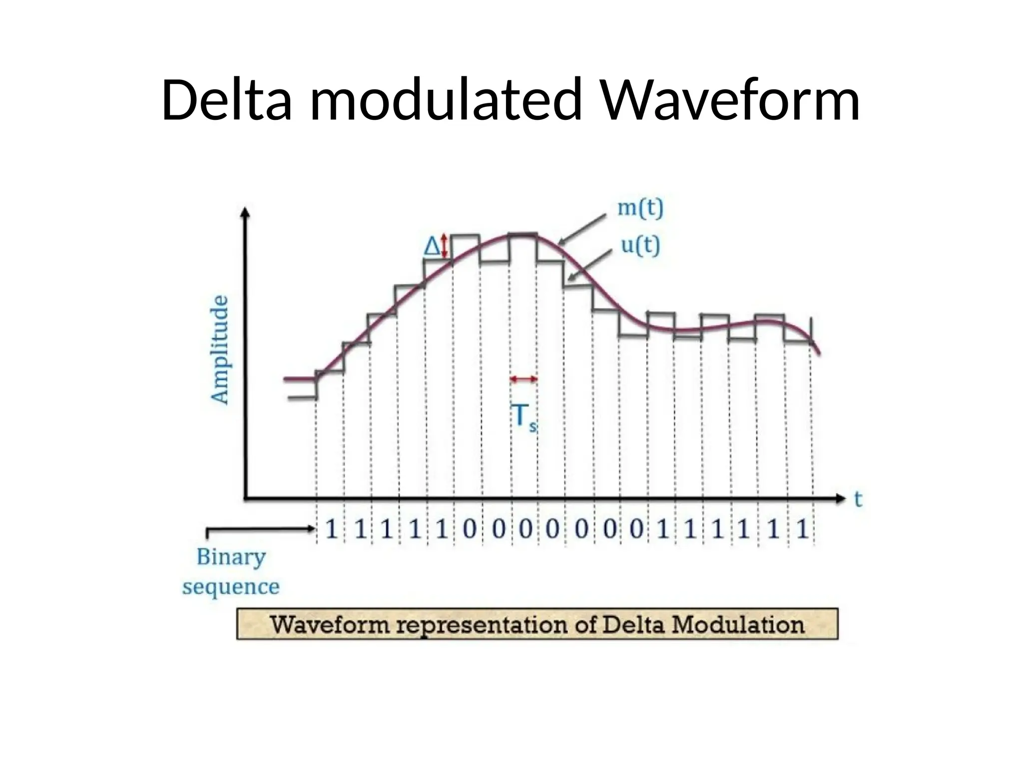
• In the end, depending on the staircase signal if the step size is +Δ
then binary 1 is transmitted and if it is –Δ then binary 0 is
transmitted.
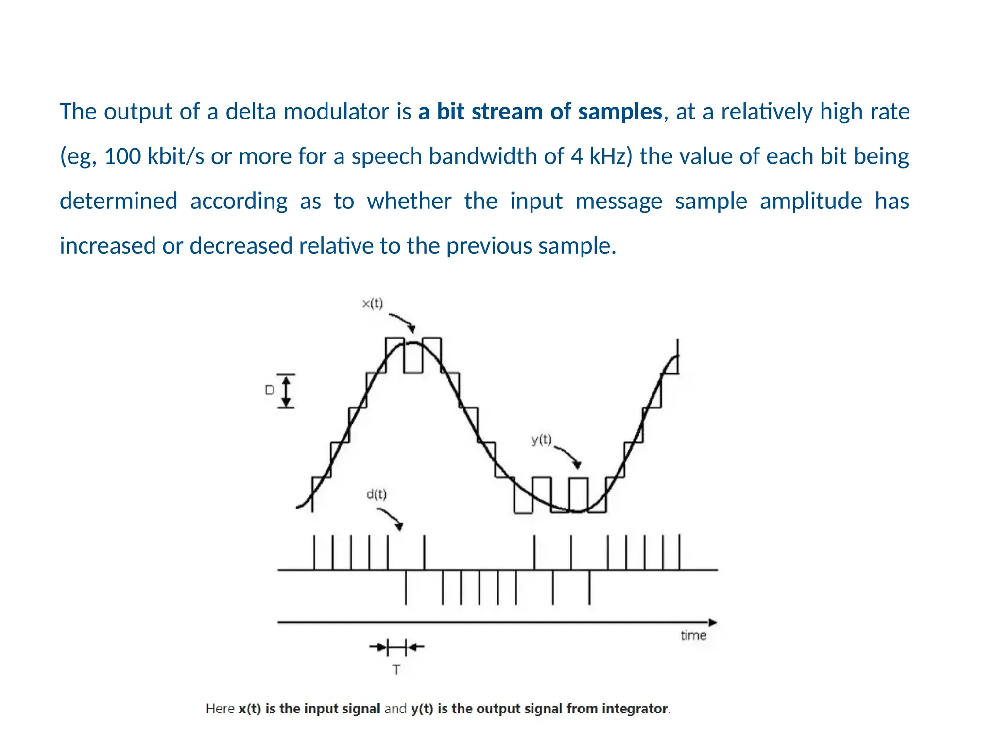
The output ofa delta modulator is a bit stream of samples, at a relatively high rate
(eg, 100 kbit/s or more for a speech bandwidth of 4 kHz) the value of each bit being
determined according as to whether the input message sample amplitude has
increased or decreased relative to the previous sample.
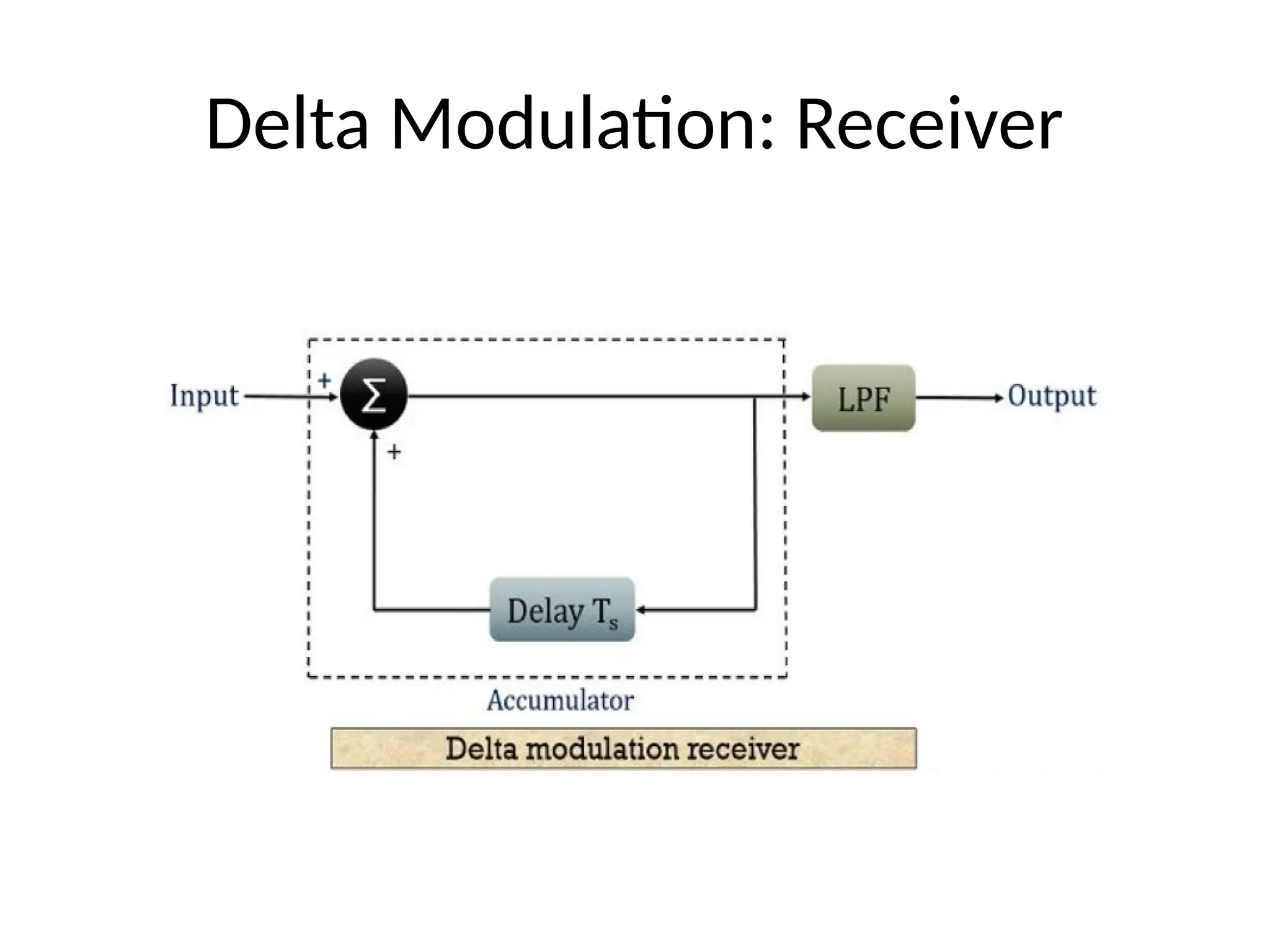
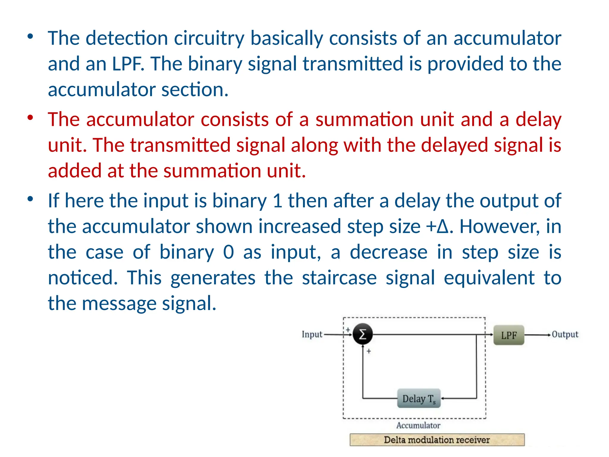
• The detectioncircuitry basically consists of an accumulator
and an LPF. The binary signal transmitted is provided to the
accumulator section.
• The accumulator consists of a summation unit and a delay
unit. The transmitted signal along with the delayed signal is
added at the summation unit.
• If here the input is binary 1 then after a delay the output of
the accumulator shown increased step size +Δ. However, in
the case of binary 0 as input, a decrease in step size is
noticed. This generates the staircase signal equivalent to
the message signal.
80.
Advantages of DM
•The advantage of delta modulation is, this
process transmits only one bit either 1 or 0
per one sample. SO it is very simple to
implement.
• So, it requires lower channel bandwidth than
the PCM & the signaling rate also small
because it generates only one bit per one
sample.
81.
Disadvantages of DM
Thedelta modulation has two major drawbacks
as under :
• Slope overload distortion
• Granular or idle noise
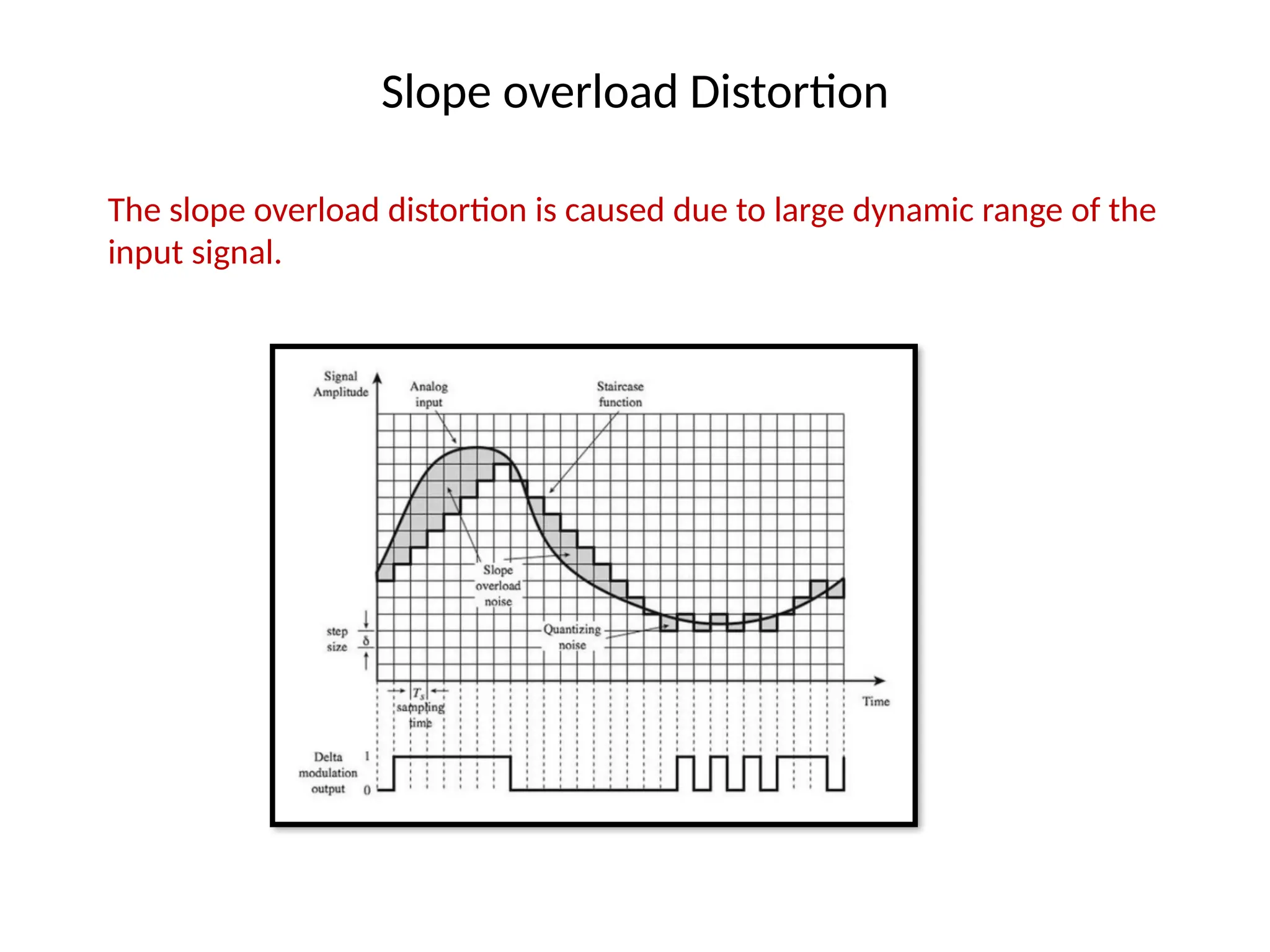
The rate ofrise of input signal x(t) is so high that the staircase signal can not follow
it or track it,.
The step size ‘Δ’ becomes too small for staircase signal u(t) to follow the step
segment of x(t).
Hence, there is a large error between the staircase approximated signal and the
original input signal x(t).
This error or noise is known as slope overload distortion .
84.
Granular Noise
• Granularor Idle noise occurs when the step size is too
large compared to small variation in the input signal.
• This means that for very small variations in the input
signal, or for constant level of signal, the staircase signal
is changed by large amount (Δ) because of large step size.
• Fig. shows that when the input signal is almost flat , the
staircase signal u(t) keeps on oscillating by ±Δ around the
signal.
• The error between the input and approximated signal is
called granular noise.
• The solution to this problem is to make the step size small
for constant or slowly varying signal.
85.
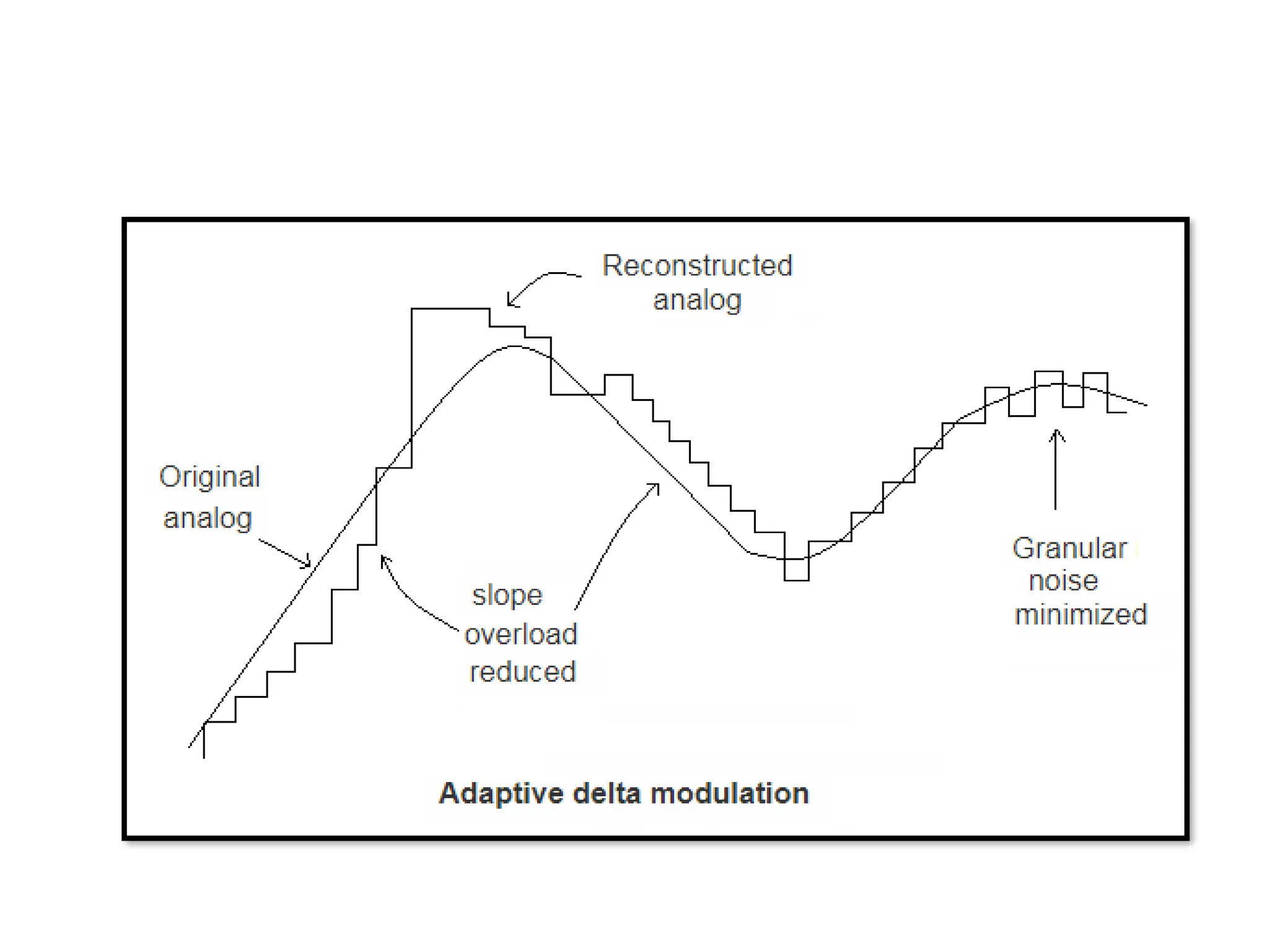
Adaptive Delta Modulation
•In order to overcome the quantization errors due to
slope overload and granular noise, the step size (Δ) is
made adaptive to variations in the input signal x(t).
• Particularly in the steep segment of the signal x(t), the
step size is increased. And the step is decreased when
the input is varying slowly.
• This method is known as Adaptive Delta Modulation
(ADM).
• The adaptive delta modulators can take continuous
changes in step size or discrete changes in step size.
88.
• Adaptive deltamodulation decreases slope
error present in delta modulation.
• During demodulation, it uses a low pass filter
which removes the quantized noise.
• The slope overload error and granular error
present in delta modulation are solved using
this modulation.

![Example: Quantization and encoding of a continuous signal with excursions from -4
Volt to +4 Volt
Step Size =[4-(-4)]/8 = 1 Volt
Eight quantization levels can
be located at :
-3.5, -2.5……+2.5, +3.5 Volt.](https://image.slidesharecdn.com/ec352dce-250320135421-5d896709/75/EC-352-DCE-Digital-Communication-Engineering-49-2048.jpg)


![Coded Agents – with UiPath SDK + LangGraph [Virtual Hands-on Workshop]](https://cdn.slidesharecdn.com/ss_thumbnails/codedagentsdeck-251215155422-5497c599-thumbnail.jpg?width=640&height=640&fit=bounds)


