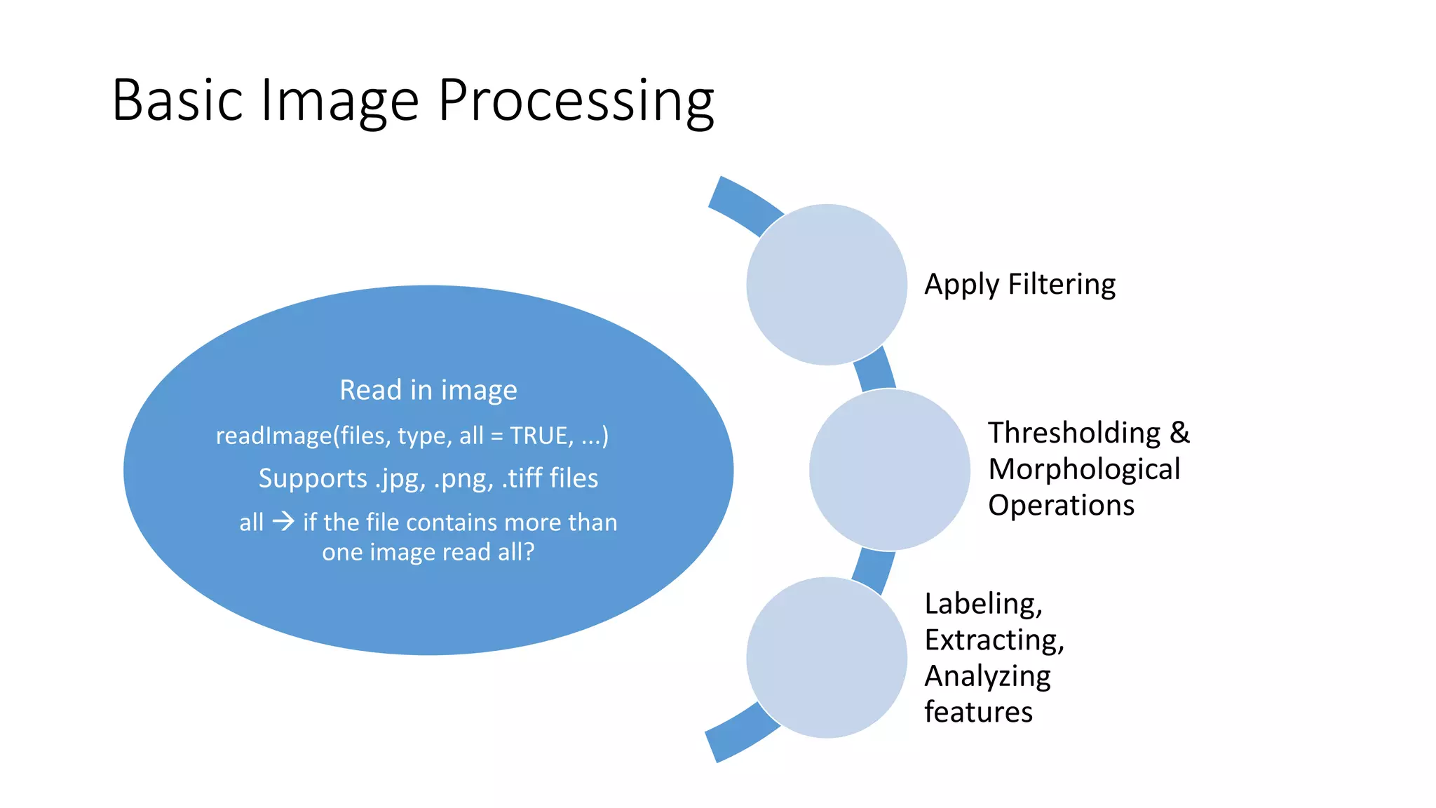
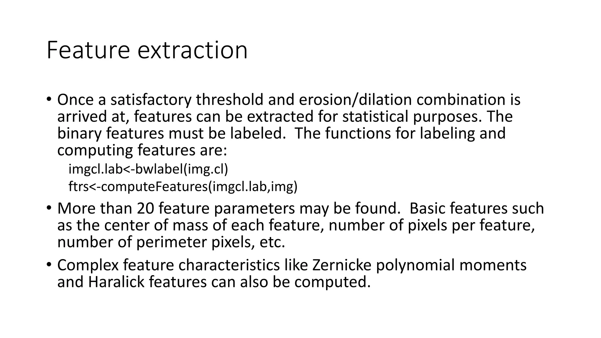
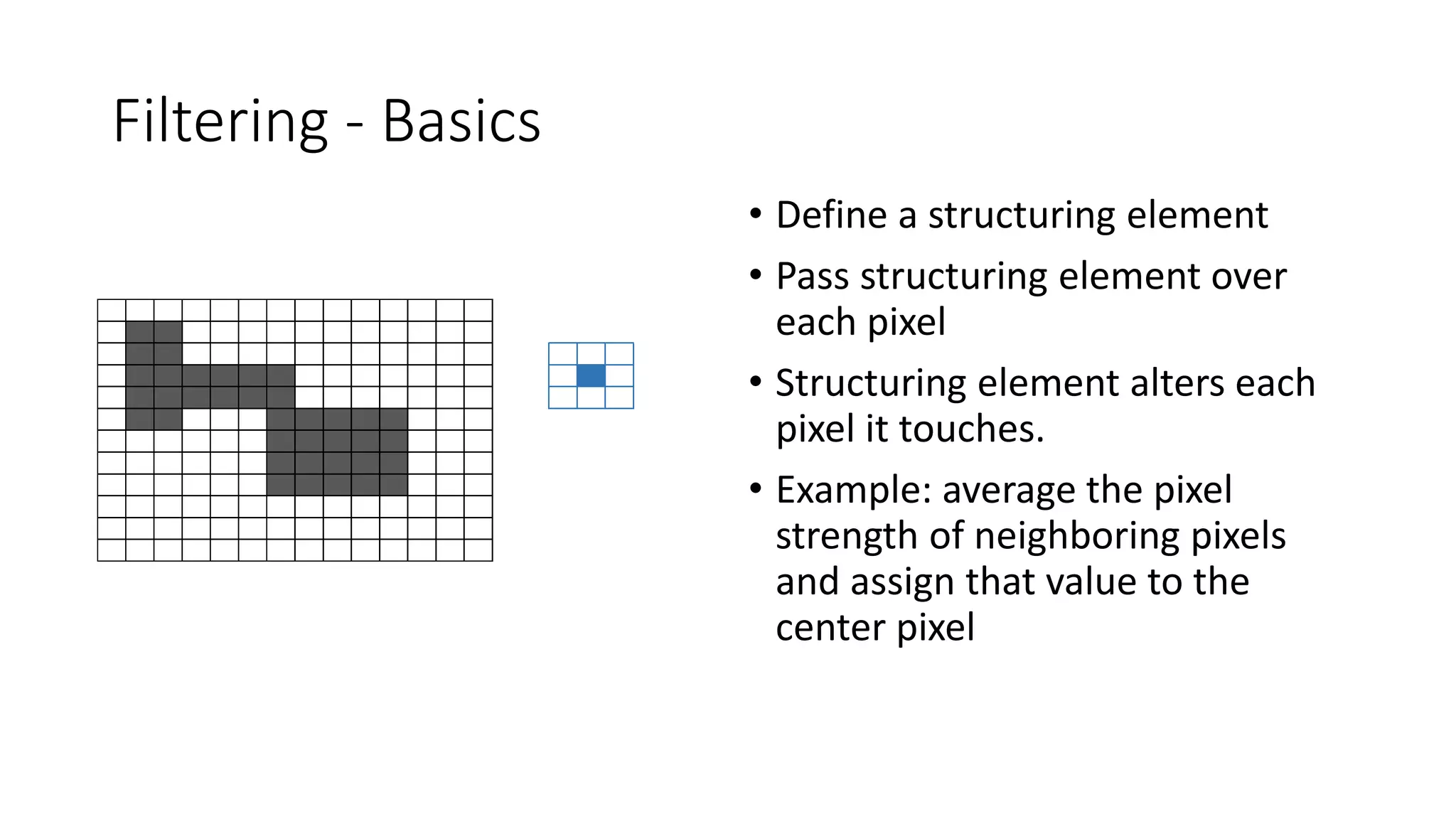
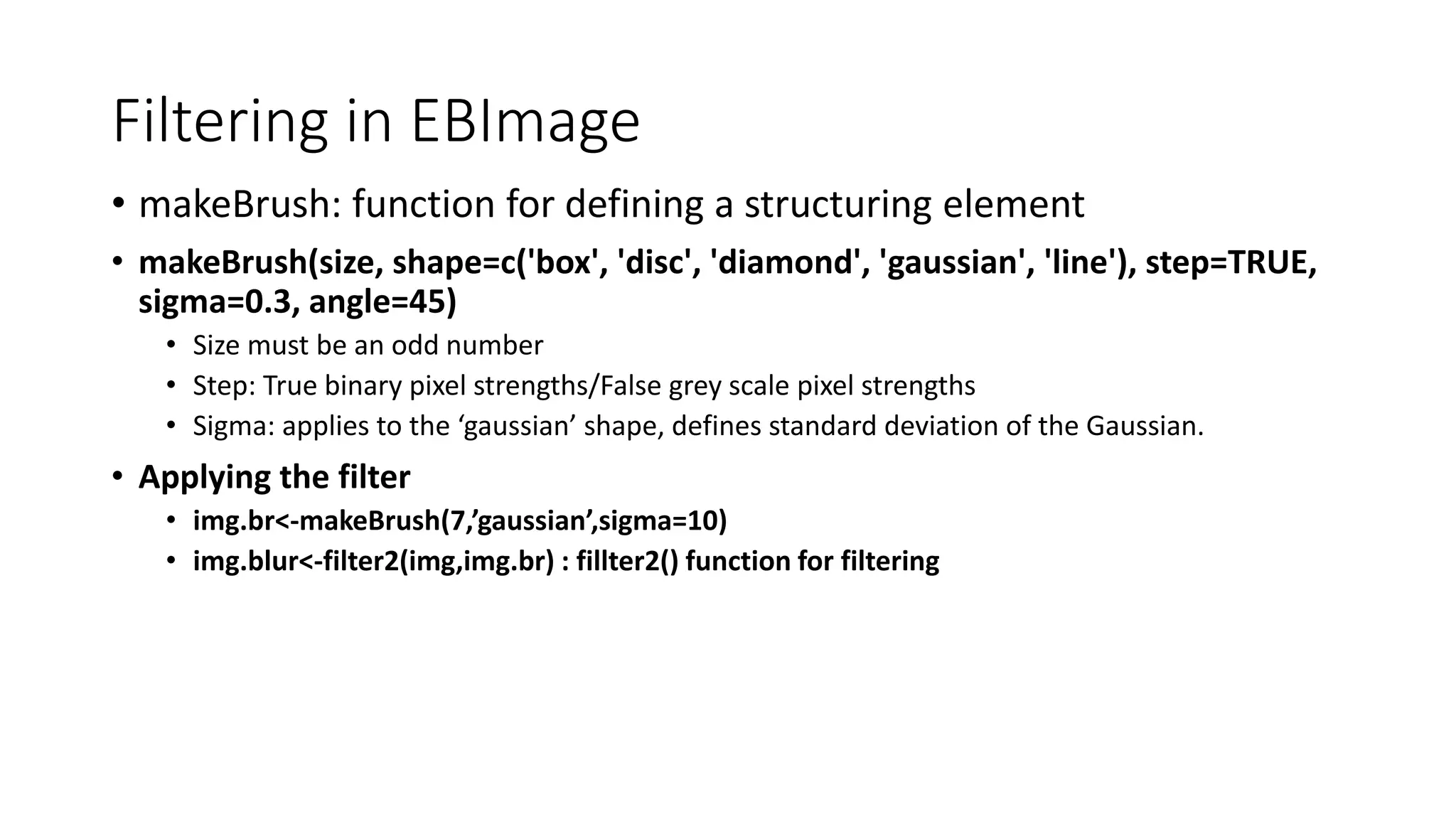
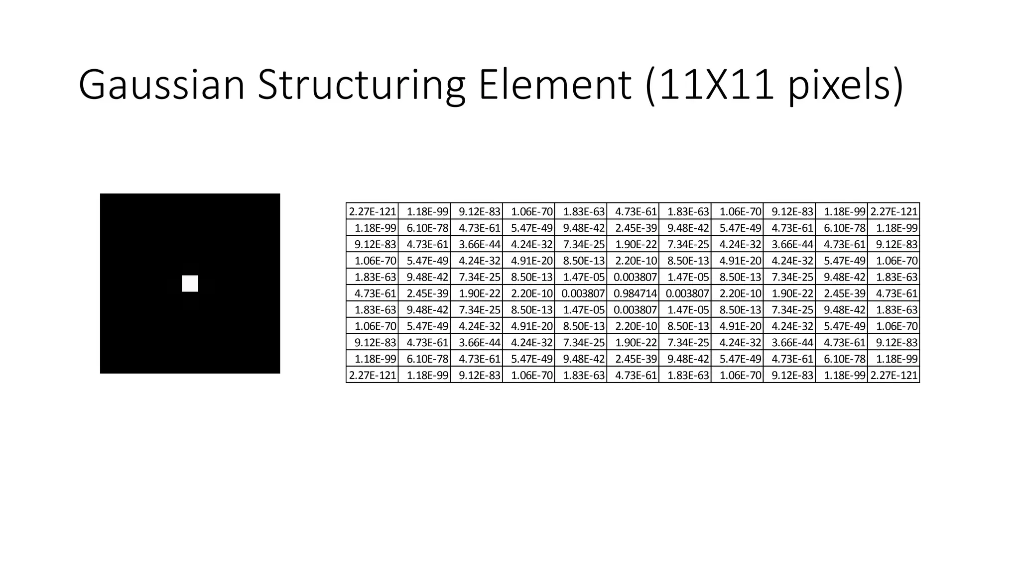
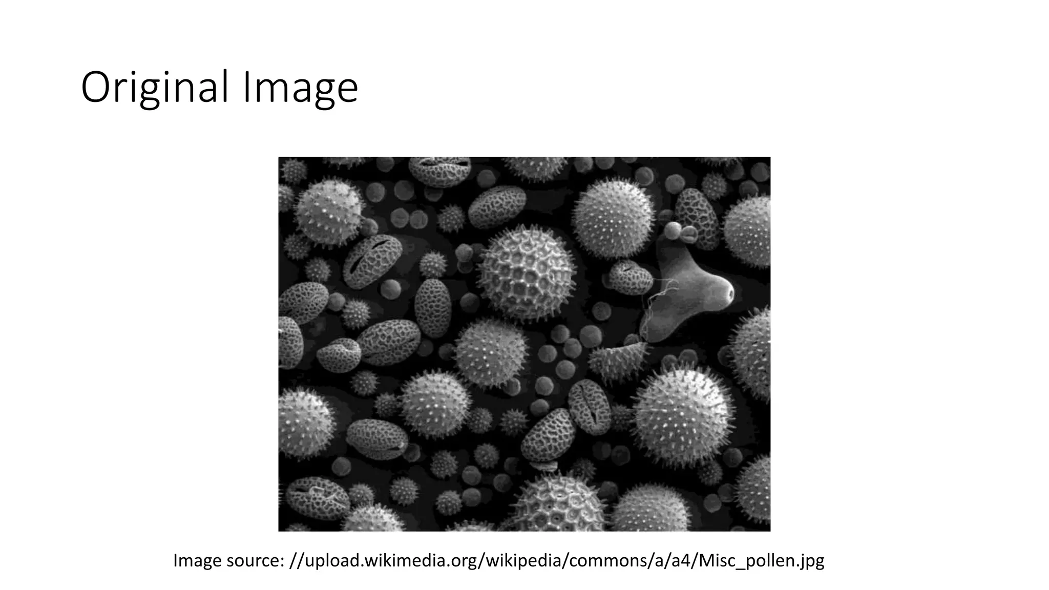
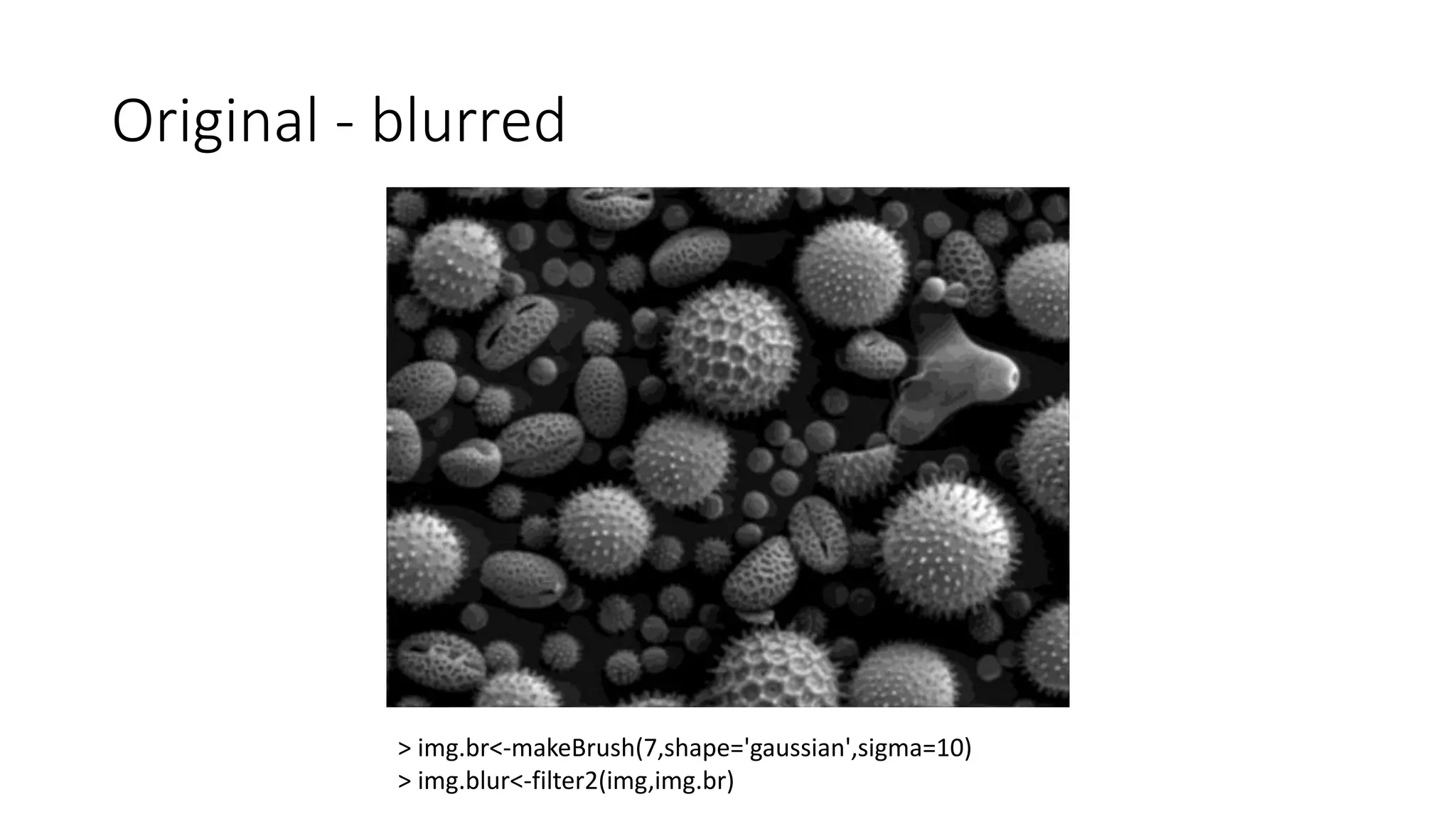
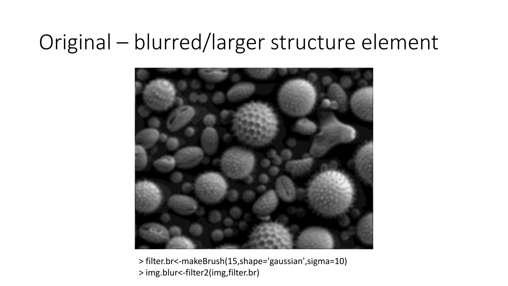
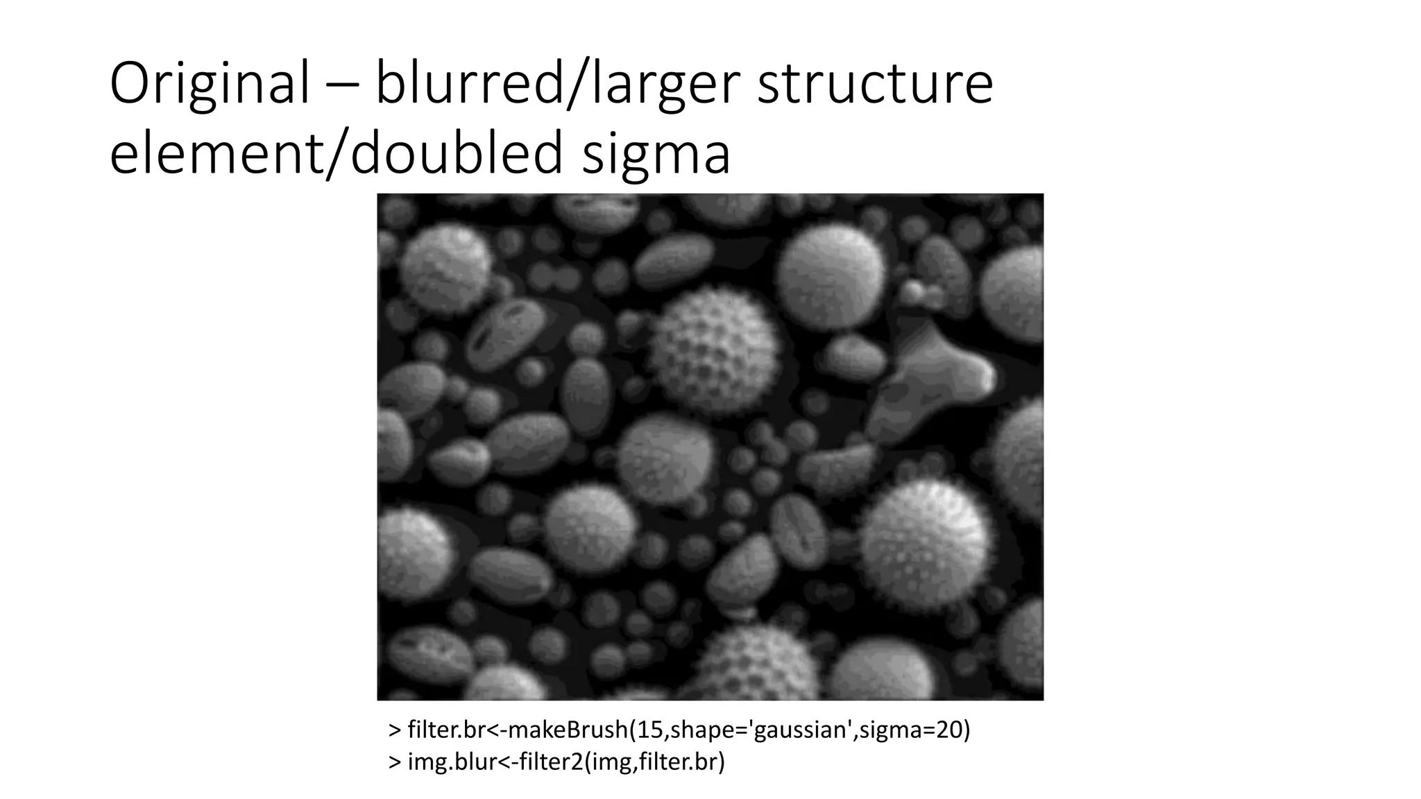
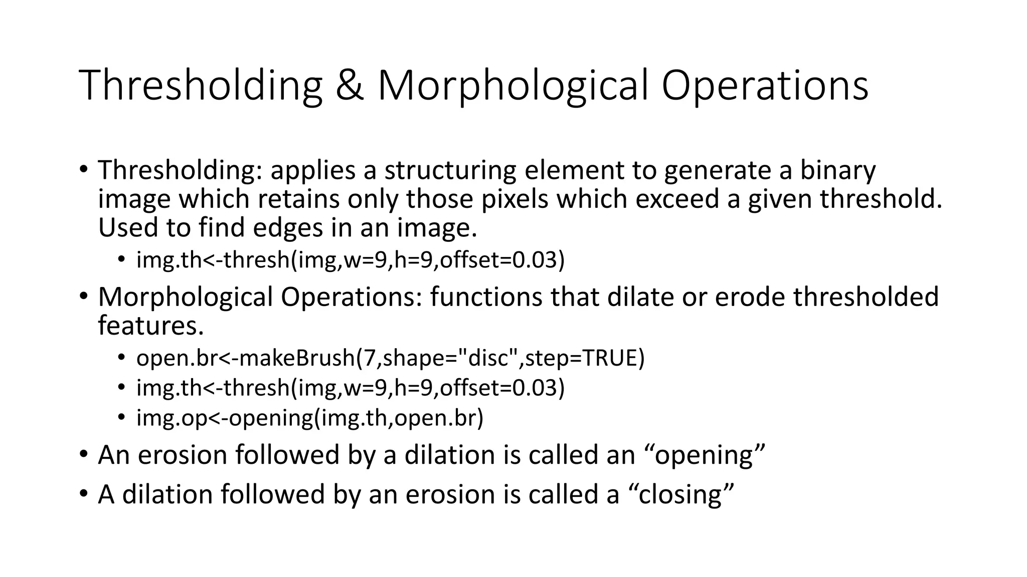
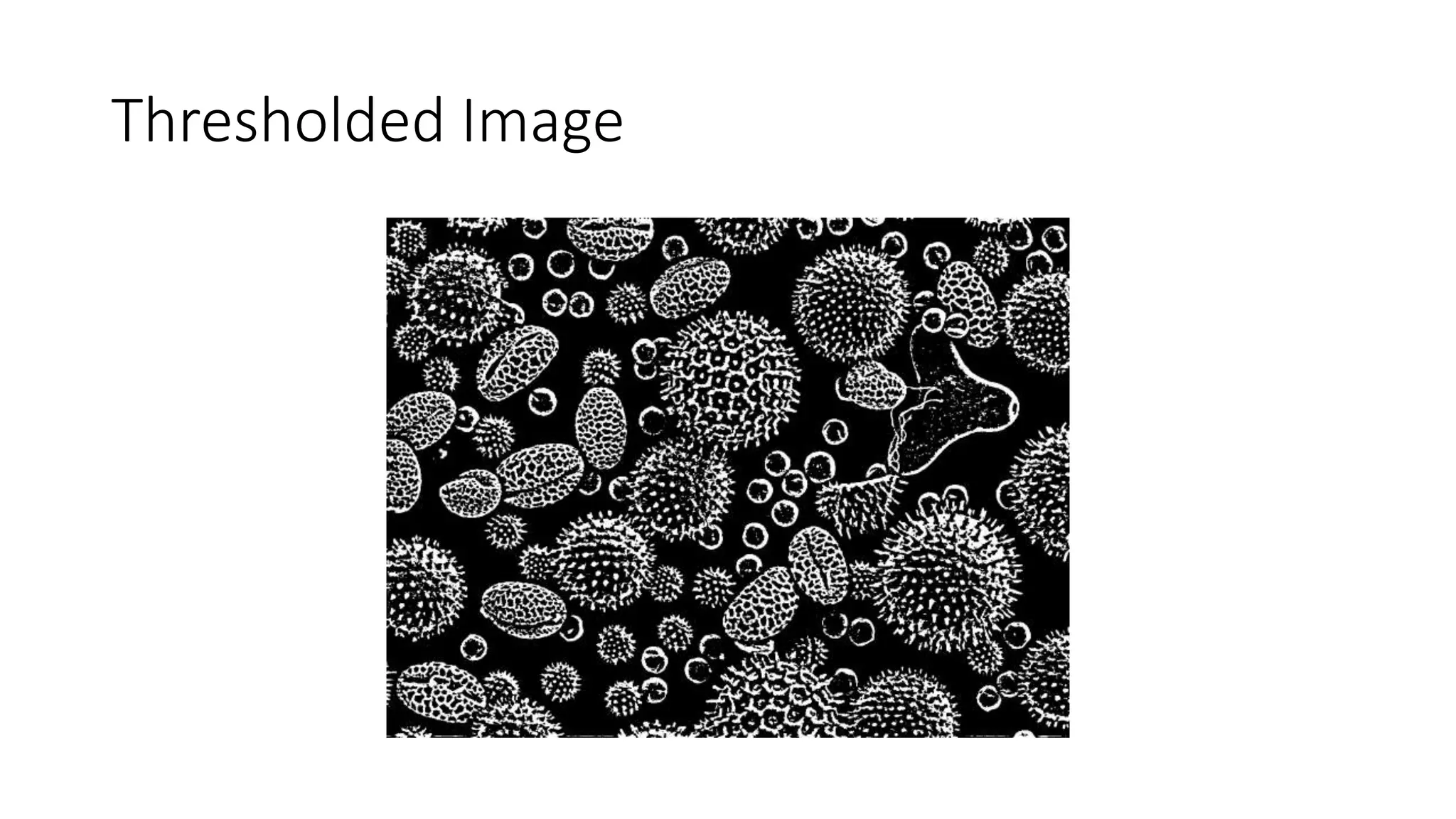
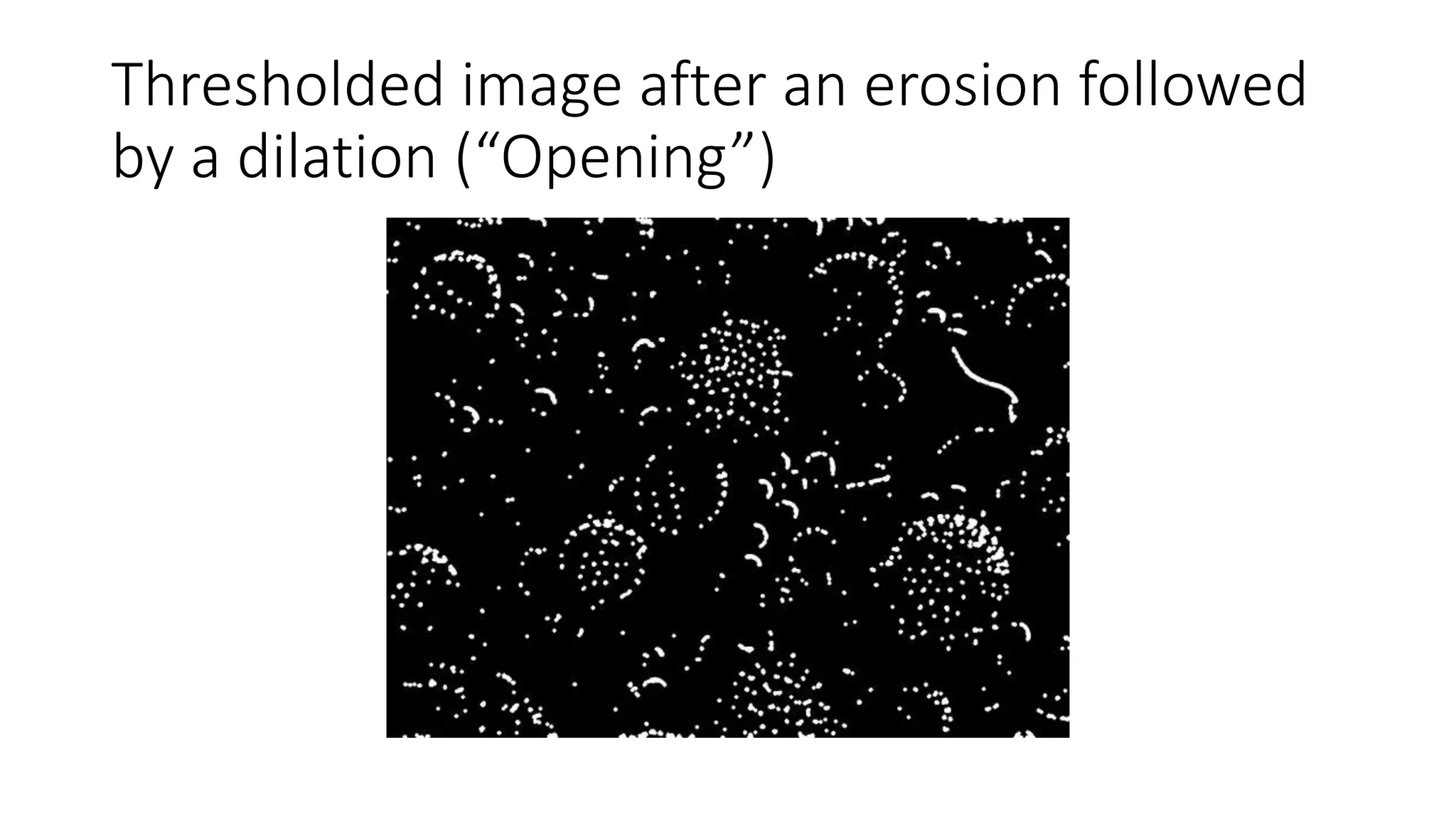
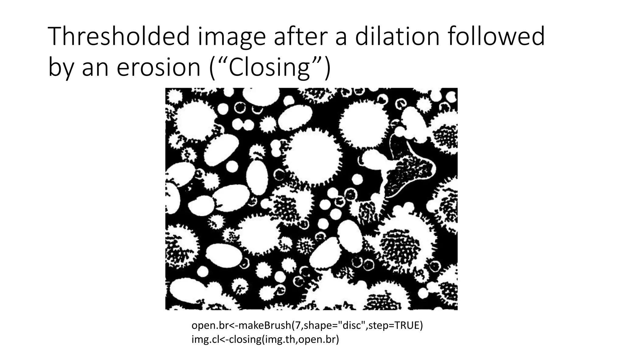
- EBImage is an image processing and analysis toolbox for R that was developed for segmenting cells and extracting quantitative descriptors - It allows users to read images, apply filters like thresholding and morphological operations, label features, and extract statistics - Filters like Gaussian blurring can be applied using structuring elements of varying sizes to smooth an image, while thresholding and morphological operations like openings and closings can be used to find edges and extract binary features for analysis

1. EBImage: Image processing
package in R
Charles Howard
Portland R Users Group
16-Sep-2015

2. EBImage
• EBImage is an image processing and analysis toolbox for R.
• Development of the package arose from the need for general purpose
tools for segmenting cells and extracting quantitative cellular
descriptors
• Package is hosted on Bioconductor (http://bioconductor.org/)
•

3. Read in image
readImage(files, type, all = TRUE, ...)
Supports .jpg, .png, .tiff files
all  if the file contains more than
one image read all?
Apply Filtering
Thresholding &
Morphological
Operations
Labeling,
Extracting,
Analyzing
features
Basic Image Processing

4. Filtering - Basics
• Define a structuring element
• Pass structuring element over
each pixel
• Structuring element alters each
pixel it touches.
• Example: average the pixel
strength of neighboring pixels
and assign that value to the
center pixel

5. Filtering in EBImage
• makeBrush: function for defining a structuring element
• makeBrush(size, shape=c('box', 'disc', 'diamond', 'gaussian', 'line'), step=TRUE,
sigma=0.3, angle=45)
• Size must be an odd number
• Step: True binary pixel strengths/False grey scale pixel strengths
• Sigma: applies to the ‘gaussian’ shape, defines standard deviation of the Gaussian.
• Applying the filter
• img.br<-makeBrush(7,’gaussian’,sigma=10)
• img.blur<-filter2(img,img.br) : fillter2() function for filtering

6. Gaussian Structuring Element (11X11 pixels)
2.27E-121 1.18E-99 9.12E-83 1.06E-70 1.83E-63 4.73E-61 1.83E-63 1.06E-70 9.12E-83 1.18E-99 2.27E-121
1.18E-99 6.10E-78 4.73E-61 5.47E-49 9.48E-42 2.45E-39 9.48E-42 5.47E-49 4.73E-61 6.10E-78 1.18E-99
9.12E-83 4.73E-61 3.66E-44 4.24E-32 7.34E-25 1.90E-22 7.34E-25 4.24E-32 3.66E-44 4.73E-61 9.12E-83
1.06E-70 5.47E-49 4.24E-32 4.91E-20 8.50E-13 2.20E-10 8.50E-13 4.91E-20 4.24E-32 5.47E-49 1.06E-70
1.83E-63 9.48E-42 7.34E-25 8.50E-13 1.47E-05 0.003807 1.47E-05 8.50E-13 7.34E-25 9.48E-42 1.83E-63
4.73E-61 2.45E-39 1.90E-22 2.20E-10 0.003807 0.984714 0.003807 2.20E-10 1.90E-22 2.45E-39 4.73E-61
1.83E-63 9.48E-42 7.34E-25 8.50E-13 1.47E-05 0.003807 1.47E-05 8.50E-13 7.34E-25 9.48E-42 1.83E-63
1.06E-70 5.47E-49 4.24E-32 4.91E-20 8.50E-13 2.20E-10 8.50E-13 4.91E-20 4.24E-32 5.47E-49 1.06E-70
9.12E-83 4.73E-61 3.66E-44 4.24E-32 7.34E-25 1.90E-22 7.34E-25 4.24E-32 3.66E-44 4.73E-61 9.12E-83
1.18E-99 6.10E-78 4.73E-61 5.47E-49 9.48E-42 2.45E-39 9.48E-42 5.47E-49 4.73E-61 6.10E-78 1.18E-99
2.27E-121 1.18E-99 9.12E-83 1.06E-70 1.83E-63 4.73E-61 1.83E-63 1.06E-70 9.12E-83 1.18E-99 2.27E-121

7. Original Image
Image source: //upload.wikimedia.org/wikipedia/commons/a/a4/Misc_pollen.jpg

8. Original - blurred
> img.br<-makeBrush(7,shape='gaussian',sigma=10)
> img.blur<-filter2(img,img.br)

9. Original – blurred/larger structure element
> filter.br<-makeBrush(15,shape='gaussian',sigma=10)
> img.blur<-filter2(img,filter.br)

10. Original – blurred/larger structure
element/doubled sigma
> filter.br<-makeBrush(15,shape='gaussian',sigma=20)
> img.blur<-filter2(img,filter.br)

11. Thresholding & Morphological Operations
• Thresholding: applies a structuring element to generate a binary
image which retains only those pixels which exceed a given threshold.
Used to find edges in an image.
• img.th<-thresh(img,w=9,h=9,offset=0.03)
• Morphological Operations: functions that dilate or erode thresholded
features.
• open.br<-makeBrush(7,shape="disc",step=TRUE)
• img.th<-thresh(img,w=9,h=9,offset=0.03)
• img.op<-opening(img.th,open.br)
• An erosion followed by a dilation is called an “opening”
• A dilation followed by an erosion is called a “closing”

12. Thresholded Image

13. Thresholded image after an erosion followed
by a dilation (“Opening”)

14. Thresholded image after a dilation followed
by an erosion (“Closing”)
open.br<-makeBrush(7,shape="disc",step=TRUE)
img.cl<-closing(img.th,open.br)

15. Feature extraction
• Once a satisfactory threshold and erosion/dilation combination is
arrived at, features can be extracted for statistical purposes. The
binary features must be labeled. The functions for labeling and
computing features are:
imgcl.lab<-bwlabel(img.cl)
ftrs<-computeFeatures(imgcl.lab,img)
• More than 20 feature parameters may be found. Basic features such
as the center of mass of each feature, number of pixels per feature,
number of perimeter pixels, etc.
• Complex feature characteristics like Zernicke polynomial moments
and Haralick features can also be computed.

16. Feature Statistics Examples
This img.cl image has 1182
individual features

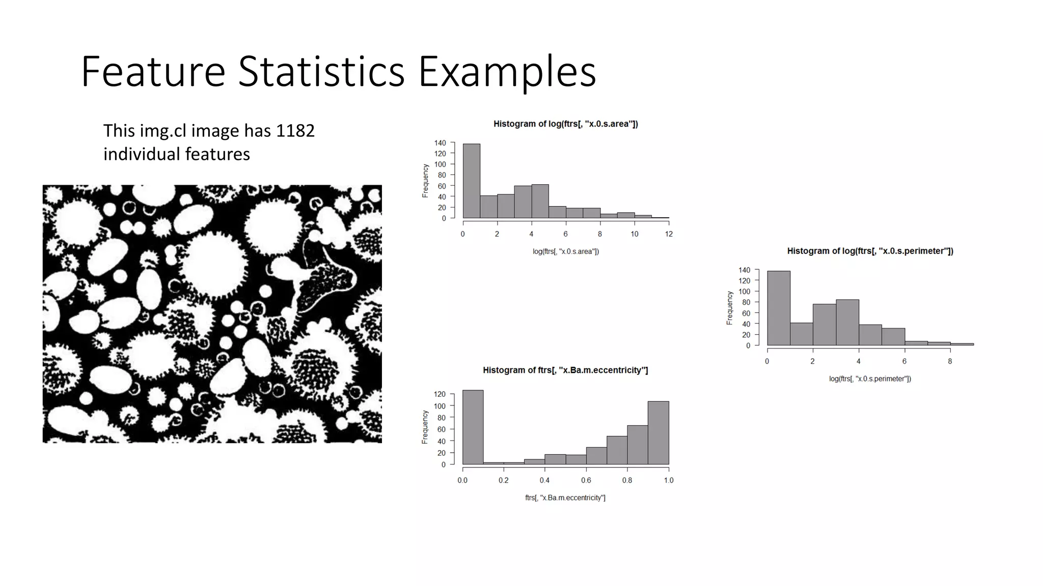
17. Feature Statistics Examples
• What are the 0.4-0.5 eccentricity features?
ecc.ftrs<-which(ftrs[,'x.a.m.eccentricity']>0.4 & ftrs[,'x.a.m.eccentricity']<=0.5)
ecc.img<-Image(0,dim=dim(img))
ecc.img[which(imgcl.lab %in% ecc.img)]<-img[which(imgcl.lab %in% ecc.img)]

18. Thanks!