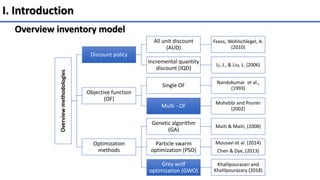
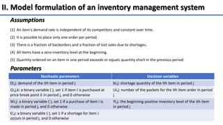
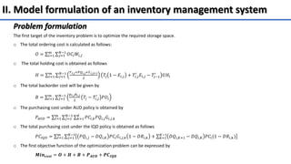
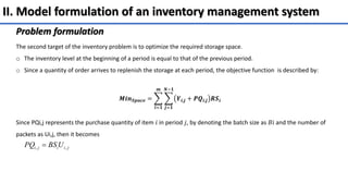
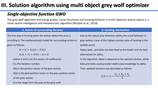
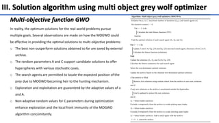
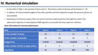
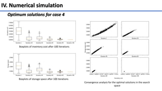
Multi-objective optimization for inventory
management systems under stochastic
demand using grey wolf optimizer
Nguyen Duy Tan
Korea Maritime & Ocean University
1. Introduction
2. Model formulation of an inventory management system
3. Solution algorithm using multi object grey wolf optimizer
4. Numerical simulation
5. Conclusion
Contents
I. Introduction
Overview inventory model
Overview
methodologies
Discount policy
All unit discount
(AUD)
Feess, Wohlschlegel, A.
(2010)
Incremental quantity
discount (IQD)
Li, J., & Liu, L. (2006)
Objective function
(OF)
Single OF
Nandakumar et al.,
(1993)
Multi - OF
Mohebbi and Posner
(2002)
Optimization
methods
Genetic algorithm
(GA)
Maiti & Maiti, (2008)
Particle swarm
optimization (PSO)
Mousavi et al. (2014)
Chen & Dye, (2013)
Grey wolf
optimization (GWO)
Khalilpourazari and
Khalilpourazary (2018)
II. Model formulation of an inventory management system
Assumptions
(1) An item's demand rate is independent of its competitors and constant over time.
(2) It is possible to place only one order per period.
(3) There is a fraction of backorders and a fraction of lost sales due to shortages.
(4) All items have a zero-inventory level at the beginning.
(5) Quantity ordered on an item in one period exceeds or equals quantity short in the previous period.
Parameters
Stochastic parameters Decision variables
Di,j: demand of the ith item in period j bi,j: shortage quantity of the ith item in period j
Gi,j,k: a binary variable ( ), set 1 if item 𝑖 is purchased at
price break point 𝑘 in period j, and 0 otherwise
Ui,j: number of the packets for the ith item order in period
j
Wi,j: a binary variable ( ), set 1 if a purchase of item i is
made in period j, and 0 otherwise
Yi,j: the beginning positive inventory level of the ith item
in period j
Ei,j: a binary variable ( ), set 1 if a shortage for item 𝑖
occurs in period j, and 0 otherwise
II. Model formulation of an inventory management system
Problem formulation
The first target of the inventory problem is to optimize the required storage space.
o The total ordering cost is calculated as follows:
𝑂 = 𝑖=1
𝑚
𝑗=1
𝑁−1
𝑂𝐶𝑖𝑊𝑖,𝑗
o The total holding cost is obtained as follows
𝐻 = 𝑖=1
𝑚
𝑗=1
𝑁−1 𝑌𝑖,𝑗+𝑃𝑄𝑖,𝑗+𝑌𝑖,𝑗+1
2
𝑇𝑗 1 − 𝐸𝑖,𝑗 + 𝑇𝑖,𝑗
′
𝐸𝑖,𝑗 − 𝑇𝑗−1
′
𝑈𝐻𝑖
o The total backorder cost will be given by
𝐵 = 𝑖=1
𝑚
𝑗=1
𝑁−1 𝑝𝑖,𝑗𝑏𝑖,𝑗
2
𝑇𝑗 − 𝑇𝑖,𝑗
′
𝑃𝑈𝑖
o The purchasing cost under AUD policy is obtained by
𝑃𝐴𝑈𝐷 = 𝐼=1
𝑚
𝑗=1
𝑁−1
𝑘=1
𝐾
𝑃𝐶𝑖,𝑘𝑃𝑄𝑖,𝑗𝐺𝑖,𝑗,𝑘
o The total purchasing cost under the IQD policy is obtained as follows
𝑃𝐶𝐼𝑄𝐷 = 𝐼=1
𝑚
𝑗=1
𝑁−1
𝑃𝑄𝑖,𝑗 − 𝐷𝑄𝑖,𝐾 𝑃𝐶𝑖𝐺𝑖,𝑗,𝑘 1 − 𝐷𝑅𝑖,𝑘 + 𝑘=1
𝐾−1
𝐷𝑄𝑖,𝐾+1 − 𝐷𝑄𝑖,𝐾 𝑃𝐶𝑖(1 − 𝐷𝑅𝑖,𝑘)
o The first objective function of the optimization problem can be expressed by
𝑴𝒊𝒏𝒄𝒐𝒔𝒕 = 𝑶 + 𝑯 + 𝑩 + 𝑷𝑨𝑼𝑫 + 𝑷𝑪𝑰𝑸𝑫
II. Model formulation of an inventory management system
Problem formulation
The second target of the inventory problem is to optimize the required storage space.
o The inventory level at the beginning of a period is equal to that of the previous period.
o Since a quantity of order arrives to replenish the storage at each period, the objective function is described by:
𝑴𝒊𝒏𝑺𝒑𝒂𝒄𝒆 =
𝒊=𝟏
𝒎
𝒋=𝟏
𝑵−𝟏
𝒀𝒊,𝒋 + 𝑷𝑸𝒊,𝒋 𝑹𝑺𝒊
Since PQi,j represents the purchase quantity of item 𝑖 in period 𝑗, by denoting the batch size as 𝐵𝑖 and the number of
packets as Ui,j, then it becomes
, ,
i j i i j
PQ BS U

III. Solution algorithm using multi object grey wolf optimizer
The grey wolf algorithm mimicking wolves' social structures and hunting behavior in multi-objective search spaces is a
novel swarm intelligence and metaheuristic algorithm (Mirjalili et al., 2014).
Single-objective function GWO
1. Action of surrounding the prey 2. Hunting mechanism
The first step in hunting when the wolves detect the prey is
encircling it. The mathematically model for surrounding actions is
given as follows:
𝐷 = 𝐶 × 𝑋𝑖 𝑘 − 𝑋(𝑘)
𝑋𝑖 𝑘 + 1 = 𝑋 𝑘 − 𝐴 × 𝐷
where A and C are the vectors of coefficients,
k is the iteration number,
X(k) is the position vector of the grey wolves,
Xi(k) is the goal position vector or the prey position vector
of the grey wolves,
D is the range from the prey to the grey wolf.
Due to the robust prey detection ability, the social behavior of
grey wolves is one of the highest success rates of hunting in the
wildlife world.
Alpha, beta , and delta are described as the leader and the best
alternatives for alpha.
In the algorithm, alpha is depicted as the optimal solution, while
beta and delta could provide helpful prey knowledge to alpha.
Their updated locations are described as follows:
𝑋 𝑘 + 1 =
𝑋𝛼 + 𝑋𝛽 + 𝑋𝛾
3
III. Solution algorithm using multi object grey wolf optimizer
Multi-objective function GWO
Algorithm: Multi object grey wolf optimizer (MOGWO)
Initialize the a, A, C, maximum number of iterations (lmax), and search agents (n)
Set iteration counter l = 0
For i = 1: n do
Calculate the total fitness function (TFF)
End for
Find the optimal solution of each search agent (Xα, Xβ, and Xδ)
For i = 1: n do
Update A and C by Eq. (24) and Eq. (25) and each search agent; Decrease a from 2 to 0;
Calculate the fitness function (solutions)
End
Update the solutions (Xα, Xβ, and Xδ) by Eq. (28)
Calculate the fitness (solutions) for each search agent
Select the non-dominated optimal solutions
Update the archive based on the obtained non-dominated optimal solutions
if the archive is filled
Remove few solutions using roulette wheel from the archive to save new solutions
end if
if any new solutions to the archive is positioned outside the hypercubes
Grid is updated to protect the new solutions
end if
Xα = Select leader (archive)
Exclude α temporarily from the archive to evade picking same leader
Xβ = Select leader (archive)
Exclude β temporarily from the archive to evade selecting same leader
Xδ = Select leader (archive). Add α and β again with the archive
l = l + 1; return the archive
In reality, the optimum solutions for the real-world problems pursue
multiple goals. Several observations are made on how the MOGWO could
be effective in providing the optimal solutions to multi-objective problems:
o The best non-outperform solutions obtained so far are saved by external
archive.
o The random parameters A and C support candidate solutions to offer
hyperspheres with various stochastic cases.
o The search agents are permitted to locate the expected position of the
prey due to MOGWO becoming heir to the hunting mechanism.
o Exploration and exploitation are guaranteed by the adaptive values of a
and A.
o Non-adaptive random values for C parameters during optimization
enhance exploration and the local front immunity of the MOGWO
algorithm concomitantly.
IV. Numerical simulation
Data Case 1 Case 2 Case 3 Case 4
m (the number of item) 10 5 15 20
N (the number of periods) 13 20 19 7
Budget limit 370000 850000 1000000 934000
K (the number of item to apply policy) 4 3 7 5
Population 50 100 200 500
Basic information for inventory optimization
o As described in Table 1, the quantity of items varies 5 - 20 and the number of periods will be between 7 - 20.
o In addition, the total available budgets of the order quantity and the breakpoints to apply the discount policies are
also provided.
o Depending on the business goals, there are several inventory model properties that might be useful in the
optimization objective. A multi-objective GWO algorithm can provide the (near)-optimum solutions.
IV. Numerical simulation
Optimum solutions for four different scenarios
Optimal solutions Case 1 Case 2 Case 3 Case 4 Mean St. Dev
Inventory cost (USD) 107743 86079 347822 140305 170487 104188
Storage space (m2) 5235 4865 8336 11833 7567 2808
TFF (𝛌 = 𝝁 = 1) 112978 90944 356158 152183 178066 105135
o Table above shows the test results on the optimal solutions for each objective function aiming at the point of
convergence.
o In this simulation, the different weights (𝛌 , 𝝁) are employed for the calculation of the total fitness function (TFF)
which describes the weighted sum of two objective
IV. Numerical simulation
Results explanation case 1
Boxplots of inventory cost after 100 iterations
o The box extends from the lower to upper quartile values of the data, with a line at the median.
o The whiskers extend from the box to show the range of the data.
o Flier points are those past the end of the whiskers.
IV. Numerical simulation
Results explanation case 1
o As can be seen in the first iteration, 100 solutions are
randomly generated based on the parameters
specified in Algorithm, and they are scatterly
distributed.
o At this stage, a set of solutions does not indicate the
optimum, like a pack of wolves starting to search for
preys.
o After 20, 40, 60, and 80 iterations, the solutions
gradually converge to a specific region as wolves
finally catch their preys, as demonstrated in the
100th iteration.
o Then, the convergence point is considered as the
(near) -optimal solution for this case.
Convergence analysis for the optimal solutions in the search
space
IV. Numerical simulation
Optimum solutions for case 2
Boxplots of inventory cost after 100 iterations
Boxplots of storage space after 100 iterations
Convergence analysis for the optimal solutions in the search
space
IV. Numerical simulation
Optimum solutions for case 3
Boxplots of inventory cost after 100 iterations
Boxplots of storage space after 100 iterations
Convergence analysis for the optimal solutions in the search
space
IV. Numerical simulation
Optimum solutions for case 4
Boxplots of inventory cost after 100 iterations
Boxplots of storage space after 100 iterations
Convergence analysis for the optimal solutions in the search
space
V. Conclusion
o In this article, a multi-item multi-period inventory management model under the limited budget with stochastic
event is presented with multiple goals of optimizing the inventory cost and storage space.
o The multiple goals are to minimize both the total costs of inventory and the required storage space.
o The purpose of the study is to determine the optimal order quantity and shortage quantity of each product in each
period so that the objective functions are optimized with the constraints.
o The developed model is an integer nonlinear programming model mixed with binary variables, and the multi-
objective optimization algorithms have been applied to solve the inventory management problem.
o Finally, the proposed leader selection mechanism allows the MOGWO algorithm to guarantee superior coverage and
convergence simultaneously.
o For specific real-word situation, real data can be employed to explore more practical marketing scenarios, and a
comparison to other meta-heuristic algorithms should be considered in the future.
Thank you for
your listening

Duy Tan NGUYEN_Multi-objective optimization for inventory management systems under stochastic demand using grey wolf optimizer.pptx

  • 1.
    Multi-objective optimization forinventory management systems under stochastic demand using grey wolf optimizer Nguyen Duy Tan Korea Maritime & Ocean University
  • 2.
    1. Introduction 2. Modelformulation of an inventory management system 3. Solution algorithm using multi object grey wolf optimizer 4. Numerical simulation 5. Conclusion Contents
  • 3.
    I. Introduction Overview inventorymodel Overview methodologies Discount policy All unit discount (AUD) Feess, Wohlschlegel, A. (2010) Incremental quantity discount (IQD) Li, J., & Liu, L. (2006) Objective function (OF) Single OF Nandakumar et al., (1993) Multi - OF Mohebbi and Posner (2002) Optimization methods Genetic algorithm (GA) Maiti & Maiti, (2008) Particle swarm optimization (PSO) Mousavi et al. (2014) Chen & Dye, (2013) Grey wolf optimization (GWO) Khalilpourazari and Khalilpourazary (2018)
  • 4.
    II. Model formulationof an inventory management system Assumptions (1) An item's demand rate is independent of its competitors and constant over time. (2) It is possible to place only one order per period. (3) There is a fraction of backorders and a fraction of lost sales due to shortages. (4) All items have a zero-inventory level at the beginning. (5) Quantity ordered on an item in one period exceeds or equals quantity short in the previous period. Parameters Stochastic parameters Decision variables Di,j: demand of the ith item in period j bi,j: shortage quantity of the ith item in period j Gi,j,k: a binary variable ( ), set 1 if item 𝑖 is purchased at price break point 𝑘 in period j, and 0 otherwise Ui,j: number of the packets for the ith item order in period j Wi,j: a binary variable ( ), set 1 if a purchase of item i is made in period j, and 0 otherwise Yi,j: the beginning positive inventory level of the ith item in period j Ei,j: a binary variable ( ), set 1 if a shortage for item 𝑖 occurs in period j, and 0 otherwise
  • 5.
    II. Model formulationof an inventory management system Problem formulation The first target of the inventory problem is to optimize the required storage space. o The total ordering cost is calculated as follows: 𝑂 = 𝑖=1 𝑚 𝑗=1 𝑁−1 𝑂𝐶𝑖𝑊𝑖,𝑗 o The total holding cost is obtained as follows 𝐻 = 𝑖=1 𝑚 𝑗=1 𝑁−1 𝑌𝑖,𝑗+𝑃𝑄𝑖,𝑗+𝑌𝑖,𝑗+1 2 𝑇𝑗 1 − 𝐸𝑖,𝑗 + 𝑇𝑖,𝑗 ′ 𝐸𝑖,𝑗 − 𝑇𝑗−1 ′ 𝑈𝐻𝑖 o The total backorder cost will be given by 𝐵 = 𝑖=1 𝑚 𝑗=1 𝑁−1 𝑝𝑖,𝑗𝑏𝑖,𝑗 2 𝑇𝑗 − 𝑇𝑖,𝑗 ′ 𝑃𝑈𝑖 o The purchasing cost under AUD policy is obtained by 𝑃𝐴𝑈𝐷 = 𝐼=1 𝑚 𝑗=1 𝑁−1 𝑘=1 𝐾 𝑃𝐶𝑖,𝑘𝑃𝑄𝑖,𝑗𝐺𝑖,𝑗,𝑘 o The total purchasing cost under the IQD policy is obtained as follows 𝑃𝐶𝐼𝑄𝐷 = 𝐼=1 𝑚 𝑗=1 𝑁−1 𝑃𝑄𝑖,𝑗 − 𝐷𝑄𝑖,𝐾 𝑃𝐶𝑖𝐺𝑖,𝑗,𝑘 1 − 𝐷𝑅𝑖,𝑘 + 𝑘=1 𝐾−1 𝐷𝑄𝑖,𝐾+1 − 𝐷𝑄𝑖,𝐾 𝑃𝐶𝑖(1 − 𝐷𝑅𝑖,𝑘) o The first objective function of the optimization problem can be expressed by 𝑴𝒊𝒏𝒄𝒐𝒔𝒕 = 𝑶 + 𝑯 + 𝑩 + 𝑷𝑨𝑼𝑫 + 𝑷𝑪𝑰𝑸𝑫
  • 6.
    II. Model formulationof an inventory management system Problem formulation The second target of the inventory problem is to optimize the required storage space. o The inventory level at the beginning of a period is equal to that of the previous period. o Since a quantity of order arrives to replenish the storage at each period, the objective function is described by: 𝑴𝒊𝒏𝑺𝒑𝒂𝒄𝒆 = 𝒊=𝟏 𝒎 𝒋=𝟏 𝑵−𝟏 𝒀𝒊,𝒋 + 𝑷𝑸𝒊,𝒋 𝑹𝑺𝒊 Since PQi,j represents the purchase quantity of item 𝑖 in period 𝑗, by denoting the batch size as 𝐵𝑖 and the number of packets as Ui,j, then it becomes , , i j i i j PQ BS U 
  • 7.
    III. Solution algorithmusing multi object grey wolf optimizer The grey wolf algorithm mimicking wolves' social structures and hunting behavior in multi-objective search spaces is a novel swarm intelligence and metaheuristic algorithm (Mirjalili et al., 2014). Single-objective function GWO 1. Action of surrounding the prey 2. Hunting mechanism The first step in hunting when the wolves detect the prey is encircling it. The mathematically model for surrounding actions is given as follows: 𝐷 = 𝐶 × 𝑋𝑖 𝑘 − 𝑋(𝑘) 𝑋𝑖 𝑘 + 1 = 𝑋 𝑘 − 𝐴 × 𝐷 where A and C are the vectors of coefficients, k is the iteration number, X(k) is the position vector of the grey wolves, Xi(k) is the goal position vector or the prey position vector of the grey wolves, D is the range from the prey to the grey wolf. Due to the robust prey detection ability, the social behavior of grey wolves is one of the highest success rates of hunting in the wildlife world. Alpha, beta , and delta are described as the leader and the best alternatives for alpha. In the algorithm, alpha is depicted as the optimal solution, while beta and delta could provide helpful prey knowledge to alpha. Their updated locations are described as follows: 𝑋 𝑘 + 1 = 𝑋𝛼 + 𝑋𝛽 + 𝑋𝛾 3
  • 8.
    III. Solution algorithmusing multi object grey wolf optimizer Multi-objective function GWO Algorithm: Multi object grey wolf optimizer (MOGWO) Initialize the a, A, C, maximum number of iterations (lmax), and search agents (n) Set iteration counter l = 0 For i = 1: n do Calculate the total fitness function (TFF) End for Find the optimal solution of each search agent (Xα, Xβ, and Xδ) For i = 1: n do Update A and C by Eq. (24) and Eq. (25) and each search agent; Decrease a from 2 to 0; Calculate the fitness function (solutions) End Update the solutions (Xα, Xβ, and Xδ) by Eq. (28) Calculate the fitness (solutions) for each search agent Select the non-dominated optimal solutions Update the archive based on the obtained non-dominated optimal solutions if the archive is filled Remove few solutions using roulette wheel from the archive to save new solutions end if if any new solutions to the archive is positioned outside the hypercubes Grid is updated to protect the new solutions end if Xα = Select leader (archive) Exclude α temporarily from the archive to evade picking same leader Xβ = Select leader (archive) Exclude β temporarily from the archive to evade selecting same leader Xδ = Select leader (archive). Add α and β again with the archive l = l + 1; return the archive In reality, the optimum solutions for the real-world problems pursue multiple goals. Several observations are made on how the MOGWO could be effective in providing the optimal solutions to multi-objective problems: o The best non-outperform solutions obtained so far are saved by external archive. o The random parameters A and C support candidate solutions to offer hyperspheres with various stochastic cases. o The search agents are permitted to locate the expected position of the prey due to MOGWO becoming heir to the hunting mechanism. o Exploration and exploitation are guaranteed by the adaptive values of a and A. o Non-adaptive random values for C parameters during optimization enhance exploration and the local front immunity of the MOGWO algorithm concomitantly.
  • 9.
    IV. Numerical simulation DataCase 1 Case 2 Case 3 Case 4 m (the number of item) 10 5 15 20 N (the number of periods) 13 20 19 7 Budget limit 370000 850000 1000000 934000 K (the number of item to apply policy) 4 3 7 5 Population 50 100 200 500 Basic information for inventory optimization o As described in Table 1, the quantity of items varies 5 - 20 and the number of periods will be between 7 - 20. o In addition, the total available budgets of the order quantity and the breakpoints to apply the discount policies are also provided. o Depending on the business goals, there are several inventory model properties that might be useful in the optimization objective. A multi-objective GWO algorithm can provide the (near)-optimum solutions.
  • 10.
    IV. Numerical simulation Optimumsolutions for four different scenarios Optimal solutions Case 1 Case 2 Case 3 Case 4 Mean St. Dev Inventory cost (USD) 107743 86079 347822 140305 170487 104188 Storage space (m2) 5235 4865 8336 11833 7567 2808 TFF (𝛌 = 𝝁 = 1) 112978 90944 356158 152183 178066 105135 o Table above shows the test results on the optimal solutions for each objective function aiming at the point of convergence. o In this simulation, the different weights (𝛌 , 𝝁) are employed for the calculation of the total fitness function (TFF) which describes the weighted sum of two objective
  • 11.
    IV. Numerical simulation Resultsexplanation case 1 Boxplots of inventory cost after 100 iterations o The box extends from the lower to upper quartile values of the data, with a line at the median. o The whiskers extend from the box to show the range of the data. o Flier points are those past the end of the whiskers.
  • 12.
    IV. Numerical simulation Resultsexplanation case 1 o As can be seen in the first iteration, 100 solutions are randomly generated based on the parameters specified in Algorithm, and they are scatterly distributed. o At this stage, a set of solutions does not indicate the optimum, like a pack of wolves starting to search for preys. o After 20, 40, 60, and 80 iterations, the solutions gradually converge to a specific region as wolves finally catch their preys, as demonstrated in the 100th iteration. o Then, the convergence point is considered as the (near) -optimal solution for this case. Convergence analysis for the optimal solutions in the search space
  • 13.
    IV. Numerical simulation Optimumsolutions for case 2 Boxplots of inventory cost after 100 iterations Boxplots of storage space after 100 iterations Convergence analysis for the optimal solutions in the search space
  • 14.
    IV. Numerical simulation Optimumsolutions for case 3 Boxplots of inventory cost after 100 iterations Boxplots of storage space after 100 iterations Convergence analysis for the optimal solutions in the search space
  • 15.
    IV. Numerical simulation Optimumsolutions for case 4 Boxplots of inventory cost after 100 iterations Boxplots of storage space after 100 iterations Convergence analysis for the optimal solutions in the search space
  • 16.
    V. Conclusion o Inthis article, a multi-item multi-period inventory management model under the limited budget with stochastic event is presented with multiple goals of optimizing the inventory cost and storage space. o The multiple goals are to minimize both the total costs of inventory and the required storage space. o The purpose of the study is to determine the optimal order quantity and shortage quantity of each product in each period so that the objective functions are optimized with the constraints. o The developed model is an integer nonlinear programming model mixed with binary variables, and the multi- objective optimization algorithms have been applied to solve the inventory management problem. o Finally, the proposed leader selection mechanism allows the MOGWO algorithm to guarantee superior coverage and convergence simultaneously. o For specific real-word situation, real data can be employed to explore more practical marketing scenarios, and a comparison to other meta-heuristic algorithms should be considered in the future.
  • 17.