3
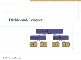
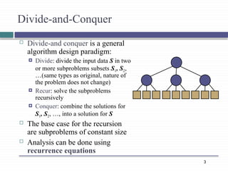
Divide-and-Conquer
Divide-and conqueris a general
algorithm design paradigm:
Divide: divide the input data S in two
or more subproblems subsets S1, S2,
…(same types as original, nature of
the problem does not change)
Recur: solve the subproblems
recursively
Conquer: combine the solutions for
S1, S2, …, into a solution for S
The base case for the recursion
are subproblems of constant size
Analysis can be done using
recurrence equations
5
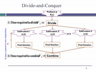
Divide-and-Conquer
+
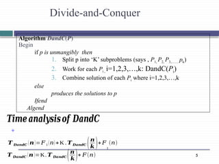
𝑻 𝑫𝒂𝒏𝒅𝑪 (𝒏)=𝐹1(𝑛)+K . 𝑻𝑫𝒂𝒏𝒅𝑪 (𝒏
𝒌 )+𝐹
1
(𝑛)
𝑻 𝑫𝒂𝒏𝒅𝑪 (𝒏)=K.𝑻 𝑫𝒂𝒏𝒅𝑪 (𝒏
𝒌)+ 𝐹(𝑛)
Algorithm DandC(P)
Begin
if p is unmangibly then
1. Split p into ‘K’ subproblems (says , P1, P2, P3,…… pk)
2. Work for each Pi , i=1,2,3,…,k: DandC(Pi)
3. Combine solution of each Pi where i=1,2,3,…,k
else
produces the solutions to p
Ifend
Algend
𝑻𝒊𝒎𝒆𝒂𝒏𝒂𝒍𝒚𝒔𝒊𝒔𝒐𝒇 𝑫𝒂𝒏𝒅𝑪
7
CSE 353– Lecture3
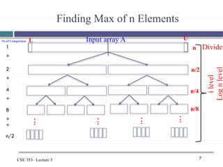
Finding Max of n Elements
Divide
Input array A
i
level
Log
n
level
n
n/2
.
.
.
.
.
.
.
.
.
.
.
.
n/8
n/4
1
+
2
+
4
+
8
+
+
n/2
No of Comparison L U
8.
8
Algorithm Max (A,L, U)
if L = U then
return A[L]
else
mid (L+U)/2; (Divide)
M1=Max(A, L, mid); (Conquer)
M1=Max(A, mid+1, U); (Conquer)
Return (M1>M2?M1:M2);
endif
Call Merge-Sort(A,1,n) to sort A[1..n]
Recursion bottoms out when subsequences have length 1
Merge Sort
9.
9
9
=
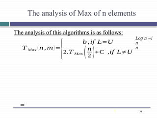
The analysis ofthis algorithms is as follows:
The analysis of Max of n elements
Log n =i
n
n
𝑇 𝑀𝑎𝑥 (𝑛, 𝑚)=
{
𝑏, 𝑖𝑓 𝐿=𝑈
2.𝑇 𝑀𝑎𝑥 (𝑛
2 )+C ,𝑖𝑓 𝐿≠𝑈
10.
10
10
6
= = =
=2[+C = 4.C
= 4.C = 8.C
= 8.C = 16.C
=16[2.C = 32.C
=
=
=
Time complexity for Tower of Hanoi Algorithm is (n)
The analysis of this algorithms is as follows:
The analysis of Max of n elements
Log n =i
n
n
.
.
.
12
CSE 353– Lecture3
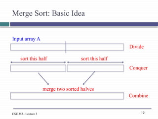
Merge Sort: Basic Idea
Divide
Input array A
Conquer
sort this half sort this half
merge two sorted halves
Combine
13.
13
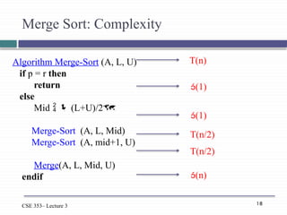
Algorithm Merge-Sort (A,L, U)
if p = r then return;
else
mid (L+U)/2; (Divide)
Merge-Sort (A, L, mid); (Conquer)
Merge-Sort (A, mid+1, U); (Conquer)
Merge (A, L, mid, U); (Combine)
endif
Call Merge-Sort(A,1,n) to sort A[1..n]
Recursion bottoms out when subsequences have length 1
Merge Sort
14.
14
CSE 353– Lecture3
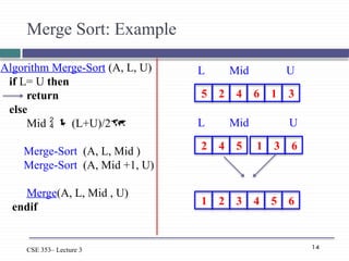
Algorithm Merge-Sort (A, L, U)
if L= U then
return
else
Mid (L+U)/2
Merge-Sort (A, L, Mid )
Merge-Sort (A, Mid +1, U)
Merge(A, L, Mid , U)
endif
Merge Sort: Example
5 2 4 6 1 3
L U
Mid
2 4 5 1 3 6
L U
Mid
1 2 3 4 5 6
15.
15
CSE 353– Lecture3
How to merge 2 sorted subarrays?
HW: Study the pseudo-code in the textbook (Sec. 2.3.1)
What is the complexity of this step? (n)
2 4 5
1 3 6
A[L..Mid]
A[Mid+1..U]
1 2 3 4 5 6
16.
16
CSE 353– Lecture3
Algorithm Merge-Sort (A, L, U)
if L = U then
return
else
Mid (L+U)/2
Merge-Sort (A, L, Mid)
Merge-Sort (A, Mid+1, U)
Merge(A, L, Mid, U)
endif
Merge Sort
Base case: L = U
Trivially correct
Inductive hypothesis: MERGE-SORT
is correct for any subarray that is a
strict (smaller) subset of A[L, Mid].
General Case: MERGE-SORT is
correct for A[L, U].
From inductive hypothesis and
correctness of Merge.
17.
17
CSE 353– Lecture3
Algorithm Merge (A, L, Mid,U)
i=L
J=Mid+1
K=L
While(i<=mid and j<=U)
if a[i]<A[j] then
B[k]=A[i]
i=i+1
else
B[k]=A[j]
j=j+1
ifend
k=k+1
whileend
Merge Sort: Correctness
If i<=mid then
For p=I to mid do
B[k]=A[p]
k=k+1
forend
else
For p= j to U do
B[k]=A[p]
k=k+1
forend
ifend
for i=L to U do
A[i]=B[i]
Forend
19
CSE 353– Lecture3
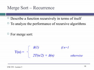
Merge Sort – Recurrence
Describe a function recursively in terms of itself
To analyze the performance of recursive algorithms
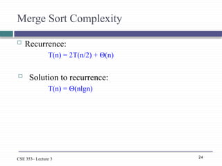
For merge sort:
(1) if n=1
2T(n/2) + (n) otherwise
T(n) =
20.
20
CSE 353– Lecture3
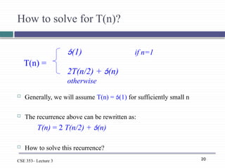
How to solve for T(n)?
Generally, we will assume T(n) = (1) for sufficiently small n
The recurrence above can be rewritten as:
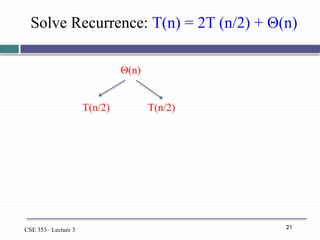
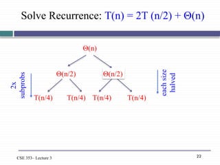
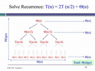
T(n) = 2 T(n/2) + (n)
How to solve this recurrence?
(1) if n=1
2T(n/2) + (n)
otherwise
T(n) =
25
CSE 353– Lecture3
Solving Recurrences
We will focus on 3 techniques in this lecture:
1. Substitution method
2. Recursion tree approach
3. Master method
26.
26
Recurrence Equation Analysis
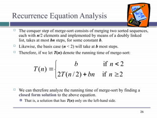
The conquer step of merge-sort consists of merging two sorted sequences,
each with n/2 elements and implemented by means of a doubly linked
list, takes at most bn steps, for some constant b.
Likewise, the basis case (n < 2) will take at b most steps.
Therefore, if we let T(n) denote the running time of merge-sort:
We can therefore analyze the running time of merge-sort by finding a
closed form solution to the above equation.
That is, a solution that has T(n) only on the left-hand side.
2
if
)
2
/
(
2
2
if
)
(
n
bn
n
T
n
b
n
T
27.
27
Iterative Substitution
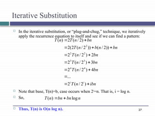
Inthe iterative substitution, or “plug-and-chug,” technique, we iteratively
apply the recurrence equation to itself and see if we can find a pattern:
Note that base, T(n)=b, case occurs when 2i
=n. That is, i = log n.
So,
Thus, T(n) is O(n log n).
ibn
n
T
bn
n
T
bn
n
T
bn
n
T
bn
n
b
n
T
bn
n
T
n
T
i
i
)
2
/
(
2
...
4
)
2
/
(
2
3
)
2
/
(
2
2
)
2
/
(
2
))
2
/
(
))
2
/
(
2
(
2
)
2
/
(
2
)
(
4
4
3
3
2
2
2
n
bn
bn
n
T log
)
(
28.
28
The Recursion Tree
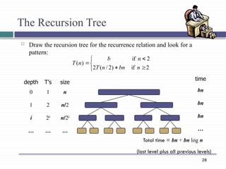
Draw the recursion tree for the recurrence relation and look for a
pattern:
depth T’s size
0 1 n
1 2 n/2
i 2i
n/2i
… … …
2
if
)
2
/
(
2
2
if
)
(
n
bn
n
T
n
b
n
T
time
bn
bn
bn
…
Total time = bn + bn log n
(last level plus all previous levels)
29.
29
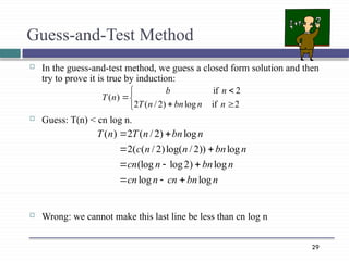
Guess-and-Test Method
Inthe guess-and-test method, we guess a closed form solution and then
try to prove it is true by induction:
Guess: T(n) < cn log n.
Wrong: we cannot make this last line be less than cn log n
n
bn
cn
n
cn
n
bn
n
cn
n
bn
n
n
c
n
bn
n
T
n
T
log
log
log
)
2
log
(log
log
))
2
/
log(
)
2
/
(
(
2
log
)
2
/
(
2
)
(
2
if
log
)
2
/
(
2
2
if
)
(
n
n
bn
n
T
n
b
n
T
30.
30
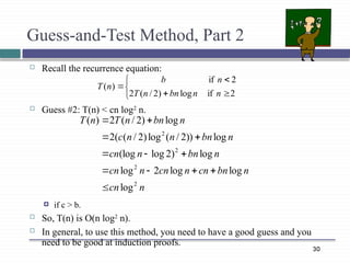
Guess-and-Test Method, Part2
Recall the recurrence equation:
Guess #2: T(n) < cn log2
n.
if c > b.
So, T(n) is O(n log2
n).
In general, to use this method, you need to have a good guess and you
need to be good at induction proofs.
n
cn
n
bn
cn
n
cn
n
cn
n
bn
n
cn
n
bn
n
n
c
n
bn
n
T
n
T
2
2
2
2
log
log
log
2
log
log
)
2
log
(log
log
))
2
/
(
log
)
2
/
(
(
2
log
)
2
/
(
2
)
(
2
if
log
)
2
/
(
2
2
if
)
(
n
n
bn
n
T
n
b
n
T
31.
31
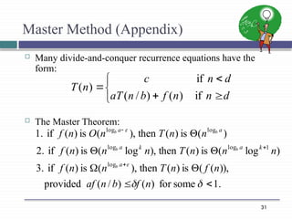
Master Method (Appendix)
Many divide-and-conquer recurrence equations have the
form:
The Master Theorem:
d
n
n
f
b
n
aT
d
n
c
n
T
if
)
(
)
/
(
if
)
(
.
1
some
for
)
(
)
/
(
provided
)),
(
(
is
)
(
then
),
(
is
)
(
if
3.
)
log
(
is
)
(
then
),
log
(
is
)
(
if
2.
)
(
is
)
(
then
),
(
is
)
(
if
1.
log
1
log
log
log
log
n
f
b
n
af
n
f
n
T
n
n
f
n
n
n
T
n
n
n
f
n
n
T
n
O
n
f
a
k
a
k
a
a
a
b
b
b
b
b
32.
32
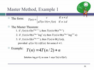
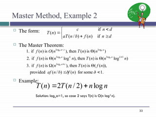
Master Method, Example1
The form:
The Master Theorem:
Example:
d
n
n
f
b
n
aT
d
n
c
n
T
if
)
(
)
/
(
if
)
(
.
1
some
for
)
(
)
/
(
provided
)),
(
(
is
)
(
then
),
(
is
)
(
if
3.
)
log
(
is
)
(
then
),
log
(
is
)
(
if
2.
)
(
is
)
(
then
),
(
is
)
(
if
1.
log
1
log
log
log
log
n
f
b
n
af
n
f
n
T
n
n
f
n
n
n
T
n
n
n
f
n
n
T
n
O
n
f
a
k
a
k
a
a
a
b
b
b
b
b
n
n
T
n
T
)
2
/
(
4
)
(
Solution: logba=2, so case 1 says T(n) is O(n2
).
33.
33
Master Method, Example2
The form:
The Master Theorem:
Example:
d
n
n
f
b
n
aT
d
n
c
n
T
if
)
(
)
/
(
if
)
(
.
1
some
for
)
(
)
/
(
provided
)),
(
(
is
)
(
then
),
(
is
)
(
if
3.
)
log
(
is
)
(
then
),
log
(
is
)
(
if
2.
)
(
is
)
(
then
),
(
is
)
(
if
1.
log
1
log
log
log
log
n
f
b
n
af
n
f
n
T
n
n
f
n
n
n
T
n
n
n
f
n
n
T
n
O
n
f
a
k
a
k
a
a
a
b
b
b
b
b
n
n
n
T
n
T log
)
2
/
(
2
)
(
Solution: logba=1, so case 2 says T(n) is O(n log2
n).
34.
34
Master Method, Example3
The form:
The Master Theorem:
Example:
d
n
n
f
b
n
aT
d
n
c
n
T
if
)
(
)
/
(
if
)
(
.
1
some
for
)
(
)
/
(
provided
)),
(
(
is
)
(
then
),
(
is
)
(
if
3.
)
log
(
is
)
(
then
),
log
(
is
)
(
if
2.
)
(
is
)
(
then
),
(
is
)
(
if
1.
log
1
log
log
log
log
n
f
b
n
af
n
f
n
T
n
n
f
n
n
n
T
n
n
n
f
n
n
T
n
O
n
f
a
k
a
k
a
a
a
b
b
b
b
b
n
n
n
T
n
T log
)
3
/
(
)
(
Solution: logba=0, so case 3 says T(n) is O(n log n).
35.
35
Master Method, Example4
The form:
The Master Theorem:
Example:
d
n
n
f
b
n
aT
d
n
c
n
T
if
)
(
)
/
(
if
)
(
.
1
some
for
)
(
)
/
(
provided
)),
(
(
is
)
(
then
),
(
is
)
(
if
3.
)
log
(
is
)
(
then
),
log
(
is
)
(
if
2.
)
(
is
)
(
then
),
(
is
)
(
if
1.
log
1
log
log
log
log
n
f
b
n
af
n
f
n
T
n
n
f
n
n
n
T
n
n
n
f
n
n
T
n
O
n
f
a
k
a
k
a
a
a
b
b
b
b
b
2
)
2
/
(
8
)
( n
n
T
n
T
Solution: logba=3, so case 1 says T(n) is O(n3
).
36.
36
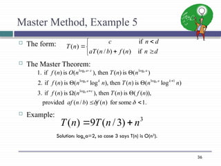
Master Method, Example5
The form:
The Master Theorem:
Example:
d
n
n
f
b
n
aT
d
n
c
n
T
if
)
(
)
/
(
if
)
(
.
1
some
for
)
(
)
/
(
provided
)),
(
(
is
)
(
then
),
(
is
)
(
if
3.
)
log
(
is
)
(
then
),
log
(
is
)
(
if
2.
)
(
is
)
(
then
),
(
is
)
(
if
1.
log
1
log
log
log
log
n
f
b
n
af
n
f
n
T
n
n
f
n
n
n
T
n
n
n
f
n
n
T
n
O
n
f
a
k
a
k
a
a
a
b
b
b
b
b
3
)
3
/
(
9
)
( n
n
T
n
T
Solution: logba=2, so case 3 says T(n) is O(n3
).
37.
37
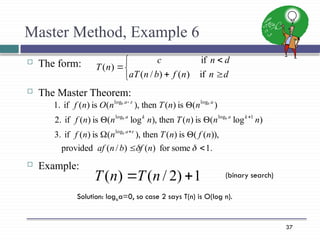
Master Method, Example6
The form:
The Master Theorem:
Example:
d
n
n
f
b
n
aT
d
n
c
n
T
if
)
(
)
/
(
if
)
(
.
1
some
for
)
(
)
/
(
provided
)),
(
(
is
)
(
then
),
(
is
)
(
if
3.
)
log
(
is
)
(
then
),
log
(
is
)
(
if
2.
)
(
is
)
(
then
),
(
is
)
(
if
1.
log
1
log
log
log
log
n
f
b
n
af
n
f
n
T
n
n
f
n
n
n
T
n
n
n
f
n
n
T
n
O
n
f
a
k
a
k
a
a
a
b
b
b
b
b
1
)
2
/
(
)
(
n
T
n
T
Solution: logba=0, so case 2 says T(n) is O(log n).
(binary search)
38.
38
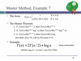
Master Method, Example7
The form:
The Master Theorem:
Example:
d
n
n
f
b
n
aT
d
n
c
n
T
if
)
(
)
/
(
if
)
(
.
1
some
for
)
(
)
/
(
provided
)),
(
(
is
)
(
then
),
(
is
)
(
if
3.
)
log
(
is
)
(
then
),
log
(
is
)
(
if
2.
)
(
is
)
(
then
),
(
is
)
(
if
1.
log
1
log
log
log
log
n
f
b
n
af
n
f
n
T
n
n
f
n
n
n
T
n
n
n
f
n
n
T
n
O
n
f
a
k
a
k
a
a
a
b
b
b
b
b
n
n
T
n
T log
)
2
/
(
2
)
(
Solution: logba=1, so case 1 says T(n) is O(n).
(heap construction)
39.
39
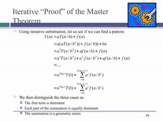
Iterative “Proof” ofthe Master
Theorem
Using iterative substitution, let us see if we can find a pattern:
We then distinguish the three cases as
The first term is dominant
Each part of the summation is equally dominant
The summation is a geometric series
1
)
(log
0
log
1
)
(log
0
log
2
2
3
3
2
2
2
)
/
(
)
1
(
)
/
(
)
1
(
.
.
.
)
(
)
/
(
)
/
(
)
/
(
)
(
)
/
(
)
/
(
))
/
(
))
/
(
(
)
(
)
/
(
)
(
n
i
i
i
a
n
i
i
i
n
b
b
b
b
b
n
f
a
T
n
b
n
f
a
T
a
n
f
b
n
af
b
n
f
a
b
n
T
a
n
f
b
n
af
b
n
T
a
bn
b
n
f
b
n
aT
a
n
f
b
n
aT
n
T
40.
40
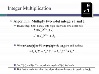
Integer Multiplication
Algorithm:Multiply two n-bit integers I and J.
Divide step: Split I and J into high-order and low-order bits
We can then define I*J by multiplying the parts and adding:
So, T(n) = 4T(n/2) + n, which implies T(n) is O(n2
).
But that is no better than the algorithm we learned in grade school.
l
n
h
l
n
h
J
J
J
I
I
I
2
/
2
/
2
2
l
l
n
h
l
n
l
h
n
h
h
l
n
h
l
n
h
J
I
J
I
J
I
J
I
J
J
I
I
J
I
2
/
2
/
2
/
2
/
2
2
2
)
2
(
*
)
2
(
*
41.
41
An Improved IntegerMultiplication Algorithm
Algorithm: Multiply two n-bit integers I and J.
Divide step: Split I and J into high-order and low-order bits
Observe that there is a different way to multiply parts:
So, T(n) = 3T(n/2) + n, which implies T(n) is O(nlog
2
3
), by the Master Theorem.
Thus, T(n) is O(n1.585
).
l
n
h
l
n
h
J
J
J
I
I
I
2
/
2
/
2
2
l
l
n
h
l
l
h
n
h
h
l
l
n
l
l
h
h
h
l
h
h
l
l
l
h
n
h
h
l
l
n
l
l
h
h
h
l
l
h
n
h
h
J
I
J
I
J
I
J
I
J
I
J
I
J
I
J
I
J
I
J
I
J
I
J
I
J
I
J
I
J
I
J
J
I
I
J
I
J
I
2
/
2
/
2
/
2
)
(
2
2
]
)
[(
2
2
]
)
)(
[(
2
*
42.
42
CSE 353– Lecture3
Solving Recurrences
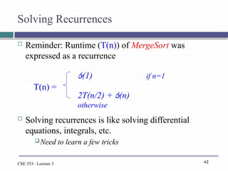
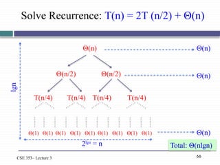
Reminder: Runtime (T(n)) of MergeSort was
expressed as a recurrence
Solving recurrences is like solving differential
equations, integrals, etc.
Need to learn a few tricks
(1) if n=1
2T(n/2) + (n)
otherwise
T(n) =
43.
43
CSE 353– Lecture3
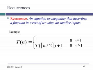
Recurrences
Recurrence: An equation or inequality that describes
a function in terms of its value on smaller inputs.
1
)
2
/
(
1
)
(
n
T
n
T if n=1
if n >1
Example:
44.
44
CSE 353– Lecture3
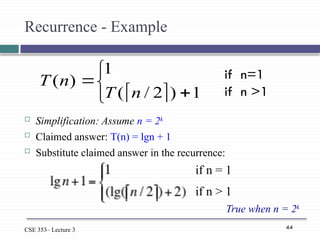
Recurrence - Example
Simplification: Assume n = 2k
Claimed answer: T(n) = lgn + 1
Substitute claimed answer in the recurrence:
1
)
2
/
(
1
)
(
n
T
n
T
if n = 1
if n > 1
True when n = 2k
if n=1
if n >1
45.
45
CSE 353– Lecture3
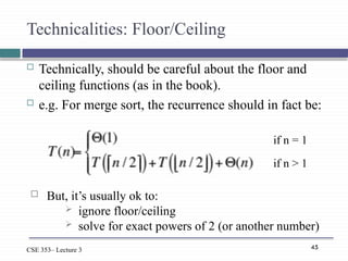
Technicalities: Floor/Ceiling
Technically, should be careful about the floor and
ceiling functions (as in the book).
e.g. For merge sort, the recurrence should in fact be:
if n = 1
if n > 1
But, it’s usually ok to:
ignore floor/ceiling
solve for exact powers of 2 (or another number)
46.
46
CSE 353– Lecture3
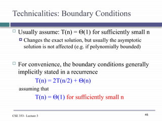
Technicalities: Boundary Conditions
Usually assume: T(n) = Θ(1) for sufficiently small n
Changes the exact solution, but usually the asymptotic
solution is not affected (e.g. if polynomially bounded)
For convenience, the boundary conditions generally
implicitly stated in a recurrence
T(n) = 2T(n/2) + Θ(n)
assuming that
T(n) = Θ(1) for sufficiently small n
47.
47
CSE 353– Lecture3
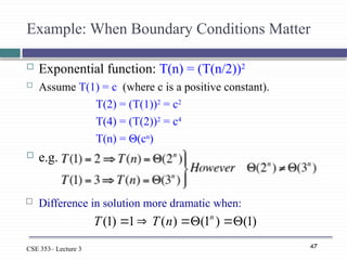
Example: When Boundary Conditions Matter
Exponential function: T(n) = (T(n/2))2
Assume T(1) = c (where c is a positive constant).
T(2) = (T(1))2
= c2
T(4) = (T(2))2
= c4
T(n) = Θ(cn
)
e.g.
)
1
(
)
1
(
)
(
1
)
1
(
n
n
T
T
Difference in solution more dramatic when:
48.
48
CSE 353– Lecture3
Solving Recurrences
We will focus on 3 techniques in this lecture:
1. Substitution method
2. Recursion tree approach
3. Master method
49.
49
CSE 353– Lecture3
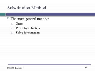
Substitution Method
The most general method:
1. Guess
2. Prove by induction
3. Solve for constants
50.
50
CSE 353– Lecture3
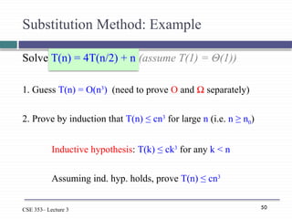
Solve T(n) = 4T(n/2) + n (assume T(1) = Θ(1))
1. Guess T(n) = O(n3
) (need to prove O and Ω separately)
2. Prove by induction that T(n) ≤ cn3
for large n (i.e. n ≥ n0)
Inductive hypothesis: T(k) ≤ ck3
for any k < n
Assuming ind. hyp. holds, prove T(n) ≤ cn3
Substitution Method: Example
51.
51
CSE 353– Lecture3
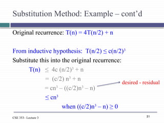
Substitution Method: Example – cont’d
Original recurrence: T(n) = 4T(n/2) + n
From inductive hypothesis: T(n/2) ≤ c(n/2)3
Substitute this into the original recurrence:
T(n) ≤ 4c (n/2)3
+ n
= (c/2) n3
+ n
= cn3
– ((c/2)n3
– n)
≤ cn3
when ((c/2)n3
– n) ≥ 0
desired - residual
52.
52
CSE 353– Lecture3
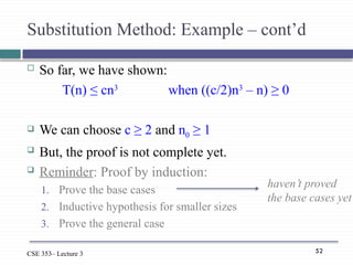
Substitution Method: Example – cont’d
So far, we have shown:
T(n) ≤ cn3
when ((c/2)n3
– n) ≥ 0
We can choose c ≥ 2 and n0 ≥ 1
But, the proof is not complete yet.
Reminder: Proof by induction:
1. Prove the base cases
2. Inductive hypothesis for smaller sizes
3. Prove the general case
haven’t proved
the base cases yet
53.
53
CSE 353– Lecture3
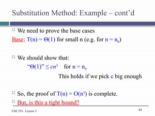
Substitution Method: Example – cont’d
We need to prove the base cases
Base: T(n) = Θ(1) for small n (e.g. for n = n0)
We should show that:
“Θ(1)” ≤ cn3
for n = n0
This holds if we pick c big enough
So, the proof of T(n) = O(n3
) is complete.
But, is this a tight bound?
54.
54
CSE 353– Lecture3
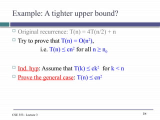
Example: A tighter upper bound?
Original recurrence: T(n) = 4T(n/2) + n
Try to prove that T(n) = O(n2
),
i.e. T(n) ≤ cn2
for all n ≥ n0
Ind. hyp: Assume that T(k) ≤ ck2
for k < n
Prove the general case: T(n) ≤ cn2
55.
55
CSE 353– Lecture3
Example (cont’d)
Original recurrence: T(n) = 4T(n/2) + n
Ind. hyp: Assume that T(k) ≤ ck2
for k < n
Prove the general case: T(n) ≤ cn2
T(n) = 4T(n/2) + n
≤ 4c(n/2)2
+ n
= cn2
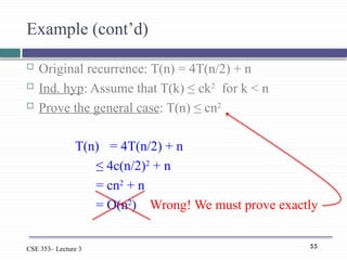
+ n
= O(n2
) Wrong! We must prove exactly
56.
56
CSE 353– Lecture3
Example (cont’d)
Original recurrence: T(n) = 4T(n/2) + n
Ind. hyp: Assume that T(k) ≤ ck2
for k < n
Prove the general case: T(n) ≤ cn2
So far, we have:
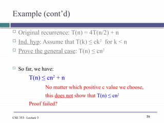
T(n) ≤ cn2
+ n
No matter which positive c value we choose,
this does not show that T(n) ≤ cn2
Proof failed?
57.
57
CSE 353– Lecture3
Example (cont’d)
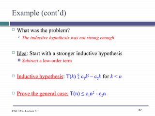
What was the problem?
The inductive hypothesis was not strong enough
Idea: Start with a stronger inductive hypothesis
Subtract a low-order term
Inductive hypothesis: T(k) c1k2
– c2k for k < n
Prove the general case: T(n) ≤ c1n2
- c2n
58.
58
CSE 353– Lecture3
Example (cont’d)
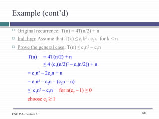
Original recurrence: T(n) = 4T(n/2) + n
Ind. hyp: Assume that T(k) ≤ c1k2
- c2k for k < n
Prove the general case: T(n) ≤ c1n2
– c2n
T(n) = 4T(n/2) + n
≤ 4 (c1(n/2)2
– c2(n/2)) + n
= c1n2
– 2c2n + n
= c1n2
– c2n – (c2n – n)
≤ c1n2
– c2n for n(c2 – 1) ≥ 0
choose c2 ≥ 1
59.
59
CSE 353– Lecture3
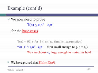
Example (cont’d)
We now need to prove
T(n) ≤ c1n2
– c2n
for the base cases.
T(n) = Θ(1) for 1 ≤ n ≤ n0 (implicit assumption)
“Θ(1)” ≤ c1n2
– c2n for n small enough (e.g. n = n0)
We can choose c1 large enough to make this hold
We have proved that T(n) = O(n2
)
60.
60
CSE 353– Lecture3
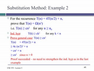
Substitution Method: Example 2
For the recurrence T(n) = 4T(n/2) + n,
prove that T(n) = Ω(n2
)
i.e. T(n) ≥ cn2
for any n ≥ n0
Ind. hyp: T(k) ≥ ck2
for any k < n
Prove general case: T(n) ≥ cn2
T(n) = 4T(n/2) + n
≥ 4c (n/2)2
+ n
= cn2
+ n
≥ cn2
since n > 0
Proof succeeded – no need to strengthen the ind. hyp as in the last
example
61.
61
CSE 353– Lecture3
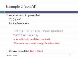
Example 2 (cont’d)
We now need to prove that
T(n) ≥ cn2
for the base cases
T(n) = Θ(1) for 1 ≤ n ≤ n0 (implicit assumption)
“Θ(1)” ≥ cn2
for n = n0
n0 is sufficiently small (i.e. constant)
We can choose c small enough for this to hold
We have proved that T(n) = Ω (n2
)
62.
62
CSE 353– Lecture3
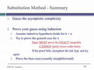
Substitution Method - Summary
1. Guess the asymptotic complexity
2. Prove your guess using induction
1. Assume inductive hypothesis holds for k < n
2. Try to prove the general case for n
Note: MUST prove the EXACT inequality
CANNOT ignore lower order terms
If the proof fails, strengthen the ind. hyp. and try
again
3. Prove the base cases (usually straightforward)
63.
63
CSE 353– Lecture3
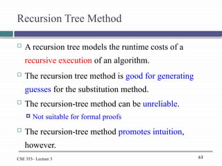
Recursion Tree Method
A recursion tree models the runtime costs of a
recursive execution of an algorithm.
The recursion tree method is good for generating
guesses for the substitution method.
The recursion-tree method can be unreliable.
Not suitable for formal proofs
The recursion-tree method promotes intuition,
however.
67
CSE 353– Lecture3
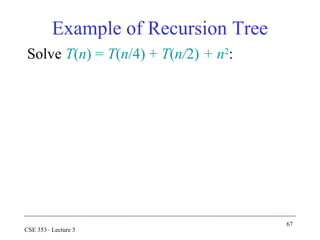
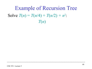
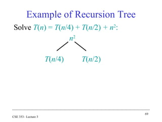
Example of Recursion Tree
Solve T(n) = T(n/4) + T(n/2) + n2
:
68.
68
CSE 353– Lecture3
Solve T(n) = T(n/4) + T(n/2) + n2
:
T(n)
Example of Recursion Tree
69.
69
CSE 353– Lecture3
Solve T(n) = T(n/4) + T(n/2) + n2
:
n2
T(n/4) T(n/2)
Example of Recursion Tree
70.
70
CSE 353– Lecture3
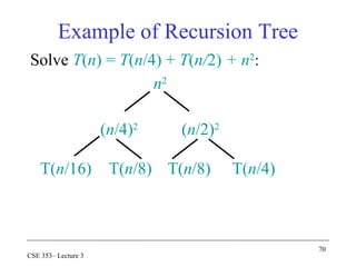
Solve T(n) = T(n/4) + T(n/2) + n2
:
n2
(n/4)2
(n/2)2
T(n/16) T(n/8) T(n/8) T(n/4)
Example of Recursion Tree
71.
71
CSE 353– Lecture3
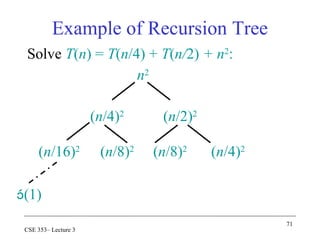
Solve T(n) = T(n/4) + T(n/2) + n2
:
n2
(n/4)2
(n/2)2
(n/16)2
(n/8)2
(n/8)2
(n/4)2
(1)
Example of Recursion Tree
72.
72
CSE 353– Lecture3
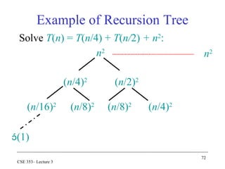
Solve T(n) = T(n/4) + T(n/2) + n2
:
n2
(n/4)2
(n/2)2
(n/16)2
(n/8)2
(n/8)2
(n/4)2
(1)
n2
Example of Recursion Tree
73.
73
CSE 353– Lecture3
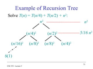
Solve T(n) = T(n/4) + T(n/2) + n2
:
n2
(n/4)2
(n/2)2
(n/16)2
(n/8)2
(n/8)2
(n/4)2
(1)
n2
5/16 n2
Example of Recursion Tree
74.
74
CSE 353– Lecture3
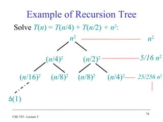
Solve T(n) = T(n/4) + T(n/2) + n2
:
n2
(n/4)2
(n/2)2
(n/16)2
(n/8)2
(n/8)2
(n/4)2
(1)
n2
5/16 n2
25/256 n2
Example of Recursion Tree
75.
75
CSE 353– Lecture3
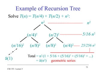
Solve T(n) = T(n/4) + T(n/2) + n2
:
n2
(n/4)2
(n/2)2
(n/16)2
(n/8)2
(n/8)2
(n/4)2
(1)
n2
5/16 n2
25/256 n2
Total = n2
(1 + 5/16 + (5/16)2
+ (5/16)3
+ ...)
= (n2
) geometric series
Example of Recursion Tree
76.
76
CSE 353– Lecture3
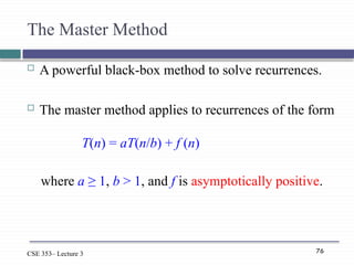
The Master Method
A powerful black-box method to solve recurrences.
The master method applies to recurrences of the form
T(n) = aT(n/b) + f (n)
where a ≥ 1, b > 1, and f is asymptotically positive.
77.
77
CSE 353– Lecture3
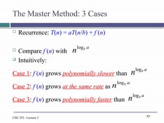
The Master Method: 3 Cases
Recurrence: T(n) = aT(n/b) + f (n)
Compare f (n) with
Intuitively:
Case 1: f (n) grows polynomially slower than
Case 2: f (n) grows at the same rate as
Case 3: f (n) grows polynomially faster than
a
b
nlog
a
b
nlog
78.
78
CSE 353– Lecture3
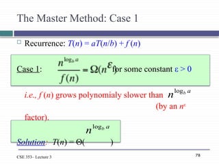
The Master Method: Case 1
Recurrence: T(n) = aT(n/b) + f (n)
Case 1: for some constant ε > 0
i.e., f (n) grows polynomialy slower than
(by an nε
factor).
Solution: T(n) = Θ( )
a
b
nlog
a
b
nlog
79.
79
CSE 353– Lecture3
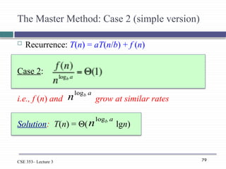
The Master Method: Case 2 (simple version)
Recurrence: T(n) = aT(n/b) + f (n)
Case 2:
i.e., f (n) and grow at similar rates
Solution: T(n) = Θ( lgn)
a
b
nlog
a
b
nlog
80.
80
CSE 353– Lecture3
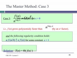
The Master Method: Case 3
Case 3: for some constant ε > 0
i.e., f (n) grows polynomialy faster than (by an nε
factor).
and the following regularity condition holds:
a f (n/b) c f (n) for some constant c < 1
Solution: T(n) = Θ( f(n) )
a
b
nlog
81.
81
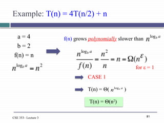
CSE 353– Lecture3
Example: T(n) = 4T(n/2) + n
a = 4
b = 2
f(n) = n
f(n) grows polynomially slower than
CASE 1
T(n) = Θ( )
a
b
nlog
T(n) = Θ(n2
)
for ε = 1
82.
82
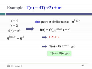
CSE 353– Lecture3
Example: T(n) = 4T(n/2) + n2
a = 4
b = 2
f(n) = n2
f(n) grows at similar rate as
CASE 2
T(n) = Θ( lgn)
a
b
nlog
T(n) = Θ(n2
lgn)
f(n) = Θ( ) = n2
83.
83
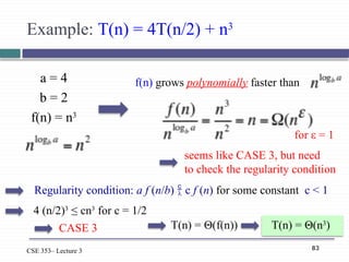
CSE 353– Lecture3
Example: T(n) = 4T(n/2) + n3
a = 4
b = 2
f(n) = n3
f(n) grows polynomially faster than
seems like CASE 3, but need
to check the regularity condition
T(n) = Θ(f(n)) T(n) = Θ(n3
)
for ε = 1
Regularity condition: a f (n/b) c f (n) for some constant c < 1
4 (n/2)3
≤ cn3
for c = 1/2
CASE 3
84.
84
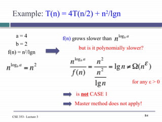
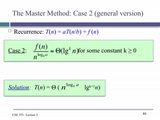
CSE 353– Lecture3
Example: T(n) = 4T(n/2) + n2
/lgn
a = 4
b = 2
f(n) = n2
/lgn
f(n) grows slower than
is not CASE 1
for any ε > 0
but is it polynomially slower?
Master method does not apply!
85.
85
CSE 353– Lecture3
The Master Method: Case 2 (general version)
Recurrence: T(n) = aT(n/b) + f (n)
Case 2: for some constant k ≥ 0
Solution: T(n) = Θ ( lgk+1
n)
a
b
nlog
86.
86
CSE 353– Lecture3
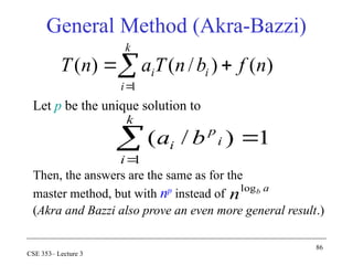
General Method (Akra-Bazzi)
Let p be the unique solution to
Then, the answers are the same as for the
master method, but with np
instead of
(Akra and Bazzi also prove an even more general result.)
k
i
i
i n
f
b
n
T
a
n
T
1
)
(
)
/
(
)
(
k
i
i
p
i b
a
1
1
)
/
(
a
b
nlog
87.
87
CSE 353– Lecture3
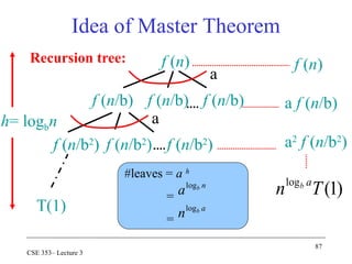
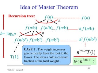
Idea of Master Theorem
Recursion tree:
)
1
(
log
T
n a
b
T(1)
f (n/b)
f (n)
f (n)
f (n/b) f (n/b)
a
a f (n/b)
f (n/b2
) f (n/b2
) f (n/b2
)
a
h= logbn
a2
f (n/b2
)
#leaves = a h
=
=
n
b
alog
a
b
nlog
88.
88
CSE 353– Lecture3
Recursion tree:
)
1
(
log
T
n a
b
T(1)
f (n/b)
f (n)
f (n)
f (n/b) f (n/b)
a
a f (n/b)
f (n/b2
) f (n/b2
) f (n/b2
)
a
h= logbn
a2
f (n/b2
)
CASE 1 : The weight increases
geometrically from the root to the
leaves. The leaves hold a constant
fraction of the total weight. Θ ( )
a
b
nlog
Idea of Master Theorem
89.
89
CSE 353– Lecture3
Recursion tree:
)
1
(
log
T
n a
b
T(1)
f (n/b)
f (n)
f (n)
f (n/b) f (n/b)
a
a f (n/b)
f (n/b2
) f (n/b2
) f (n/b2
)
a
h= logbn
a2
f (n/b2
)
CASE 2 : (k = 0) The weight
is approximately the same on
each of the logbn levels.
Θ ( lgn)
a
b
nlog
Idea of Master Theorem
90.
90
CSE 353– Lecture3
Recursion tree:
)
1
(
log
T
n a
b
T(1)
f (n/b)
f (n)
f (n)
f (n/b) f (n/b)
a
a f (n/b)
f (n/b2
) f (n/b2
) f (n/b2
)
a
h= logbn
a2
f (n/b2
)
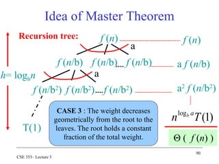
CASE 3 : The weight decreases
geometrically from the root to the
leaves. The root holds a constant
fraction of the total weight. Θ ( f (n) )
Idea of Master Theorem
91.
91
CSE 353– Lecture3
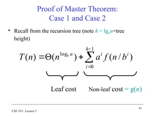
Proof of Master Theorem:
Case 1 and Case 2
• Recall from the recursion tree (note h = lgbn=tree
height)
1
0
log
)
/
(
)
(
)
(
h
i
i
i
a
b
n
f
a
n
n
T b
Leaf cost Non-leaf cost = g(n)
92.
92
CSE 353– Lecture3
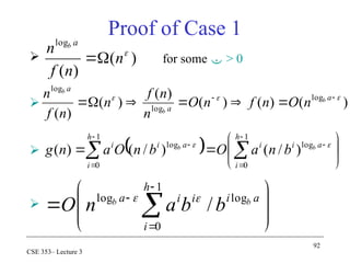
Proof of Case 1
for some > 0
)
(
)
(
log
n
n
f
n a
b
)
(
)
(
)
(
)
(
)
(
)
(
log
log
log
a
a
a
b
b
b
n
O
n
f
n
O
n
n
f
n
n
f
n
1
0
log
1
0
log
)
/
(
)
/
(
)
(
h
i
a
i
i
h
i
a
i
i b
b
b
n
a
O
b
n
O
a
n
g
1
0
log
log
/
h
i
a
i
i
i
a b
b
b
b
a
n
O
93.
93
CSE 353– Lecture3
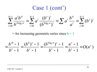
= An increasing geometric series since b > 1
1
0
1
0
log
1
0
log
)
(
)
(
)
( h
i
i
i
i
i
h
i
i
a
i
i
h
i
a
i
i
i
b
a
b
a
b
b
a
b
b
a
b
b
)
(
1
1
1
1
)
(
1
1
)
(
1
1 log
n
O
b
n
b
b
b
b
b
b n
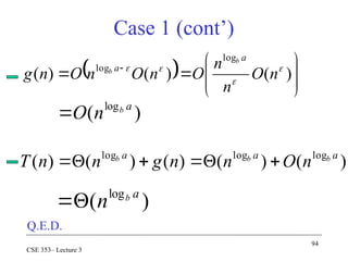
h
h b
Case 1 (cont’)
94.
94
CSE 353– Lecture3
)
(
)
(
)
(
log
log
n
O
n
n
O
n
O
n
O
n
g
a
a
b
b
)
(
)
(
)
(
)
(
)
( log
log
log a
a
a b
b
b
n
O
n
n
g
n
n
T
Case 1 (cont’)
)
( log a
b
n
O
)
( log a
b
n
Q.E.D.
95.
95
CSE 353– Lecture3
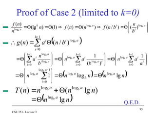
Proof of Case 2 (limited to k=0)
1
0
log
1
0
log
log
1
0
log
log
1
)
(
1 h
i
i
i
a
h
i
i
a
i
a
h
i
a
i
a
i
a
a
n
b
a
n
b
n
a b
b
b
b
b
a
i
i
a
a
b
b
b
b
n
b
n
f
n
n
f
n
n
n
f log
log
0
log
)
(
)
/
(
)
(
)
(
)
1
(
)
(lg
)
(
1
0
log
)
/
(
)
(
h
i
a
i
i b
b
n
a
n
g
)
lg
(
)
( log
log
n
n
n
n
T a
a b
b
n
n a
b
lg
log
n
n
n
n
n a
b
a
n
i
a b
b
b
b
lg
log
1 log
log
1
log
0
log
Q.E.D.
![8
Algorithm Max (A, L, U)
if L = U then
return A[L]
else
mid (L+U)/2; (Divide)
M1=Max(A, L, mid); (Conquer)
M1=Max(A, mid+1, U); (Conquer)
Return (M1>M2?M1:M2);
endif
Call Merge-Sort(A,1,n) to sort A[1..n]
Recursion bottoms out when subsequences have length 1
Merge Sort](https://image.slidesharecdn.com/lecture03-250629165035-de7808e0/85/Divided-and-conqurddddddddddddddfffffe-pptx-8-320.jpg)

![13
Algorithm Merge-Sort (A, L, U)
if p = r then return;
else
mid (L+U)/2; (Divide)
Merge-Sort (A, L, mid); (Conquer)
Merge-Sort (A, mid+1, U); (Conquer)
Merge (A, L, mid, U); (Combine)
endif
Call Merge-Sort(A,1,n) to sort A[1..n]
Recursion bottoms out when subsequences have length 1
Merge Sort](https://image.slidesharecdn.com/lecture03-250629165035-de7808e0/85/Divided-and-conqurddddddddddddddfffffe-pptx-13-320.jpg)
![15
CSE 353– Lecture 3
How to merge 2 sorted subarrays?
HW: Study the pseudo-code in the textbook (Sec. 2.3.1)
What is the complexity of this step? (n)
2 4 5
1 3 6
A[L..Mid]
A[Mid+1..U]
1 2 3 4 5 6](https://image.slidesharecdn.com/lecture03-250629165035-de7808e0/85/Divided-and-conqurddddddddddddddfffffe-pptx-15-320.jpg)
![16
CSE 353– Lecture 3
Algorithm Merge-Sort (A, L, U)
if L = U then
return
else
Mid (L+U)/2
Merge-Sort (A, L, Mid)
Merge-Sort (A, Mid+1, U)
Merge(A, L, Mid, U)
endif
Merge Sort
Base case: L = U
Trivially correct
Inductive hypothesis: MERGE-SORT
is correct for any subarray that is a
strict (smaller) subset of A[L, Mid].
General Case: MERGE-SORT is
correct for A[L, U].
From inductive hypothesis and
correctness of Merge.](https://image.slidesharecdn.com/lecture03-250629165035-de7808e0/85/Divided-and-conqurddddddddddddddfffffe-pptx-16-320.jpg)
![17
CSE 353– Lecture 3
Algorithm Merge (A, L, Mid,U)
i=L
J=Mid+1
K=L
While(i<=mid and j<=U)
if a[i]<A[j] then
B[k]=A[i]
i=i+1
else
B[k]=A[j]
j=j+1
ifend
k=k+1
whileend
Merge Sort: Correctness
If i<=mid then
For p=I to mid do
B[k]=A[p]
k=k+1
forend
else
For p= j to U do
B[k]=A[p]
k=k+1
forend
ifend
for i=L to U do
A[i]=B[i]
Forend](https://image.slidesharecdn.com/lecture03-250629165035-de7808e0/85/Divided-and-conqurddddddddddddddfffffe-pptx-17-320.jpg)


![41
An Improved Integer Multiplication Algorithm
Algorithm: Multiply two n-bit integers I and J.
Divide step: Split I and J into high-order and low-order bits
Observe that there is a different way to multiply parts:
So, T(n) = 3T(n/2) + n, which implies T(n) is O(nlog
2
3
), by the Master Theorem.
Thus, T(n) is O(n1.585
).
l
n
h
l
n
h
J
J
J
I
I
I
2
/
2
/
2
2
l
l
n
h
l
l
h
n
h
h
l
l
n
l
l
h
h
h
l
h
h
l
l
l
h
n
h
h
l
l
n
l
l
h
h
h
l
l
h
n
h
h
J
I
J
I
J
I
J
I
J
I
J
I
J
I
J
I
J
I
J
I
J
I
J
I
J
I
J
I
J
I
J
J
I
I
J
I
J
I
2
/
2
/
2
/
2
)
(
2
2
]
)
[(
2
2
]
)
)(
[(
2
*](https://image.slidesharecdn.com/lecture03-250629165035-de7808e0/85/Divided-and-conqurddddddddddddddfffffe-pptx-41-320.jpg)