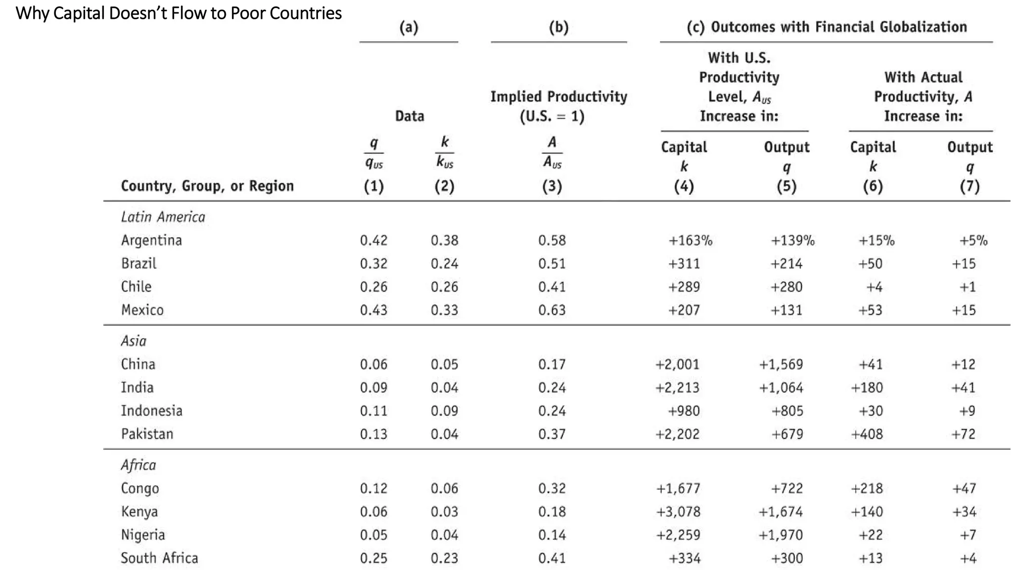
This document discusses Robert Lucas's paradox regarding why capital does not flow from rich to poor countries despite higher returns. It summarizes that: 1) Poor countries have lower productivity (different production functions) than rich countries, resulting in a smaller difference between rates of return that reduces the incentive for capital to migrate. 2) Allowing for productivity differences, investment will not cause poor countries to reach the same capital or output levels as rich countries, leading to long-run divergence rather than convergence. 3) Unless poor countries can increase productivity, greater financial integration provides limited benefits, as there are not enough opportunities for productive investment to drive complete convergence.

1. Eco 328
Divergence, diversification and demand

2. The Lucas Paradox: Why Doesn’t Capital Flow from Rich to Poor
Countries?
In his widely cited article “Why Doesn’t Capital Flow from Rich
to Poor Countries?,” Nobel laureate Robert Lucas wrote:
If this model were anywhere close to being accurate, and if
world capital markets were anywhere close to being free
and complete, it is clear that, in the face of return
differentials of this magnitude, investment goods would flow
rapidly from the United States and other wealthy countries
to India and other poor countries. Indeed, one would expect
no investment to occur in the wealthy countries. . . .
2

3. Countries Have Different Productivity Levels
To see why capital does not flow to poor countries, we now
suppose that A, the productivity level, is different in the United
States and Mexico, as denoted by country subscripts:
3

4. • The data show that Mexico’s capital per worker is about one-
third that of the United States.
• If productivity was the same, Mexico would have a level of
output level per worker of (1/3)1/3 = 0.69 or 69% of the U.S.
level. However, Mexico’s output per worker was much less,
43% of the U.S. level.
• This gap could be explained by lower productivity in Mexico.
We infer A in Mexico equals 0.43/0.69 = 62% of that in the
United States, meaning Mexico’s production function and
MPK curves are lower than those for the United States.
• The MPK gap between Mexico and the United States is much
smaller, which reduces the incentive for capital to migrate to
Mexico from the United States.
4

5. Why Doesn’t Capital Flow to Poor Countries?
This doesn’t happen in reality. Poor and rich
countries have different levels of productivity
(different production functions) and so MPK may
not be much higher in poor countries than it is in
rich countries, as shown in panel (b).
The poor country (Mexico) is now at C and not at B.
Now investment occurs only until MPK falls to the
rest of the world level at point D.
The result is divergence. Capital per worker k and
output per worker q do not converge to the levels
seen in the rich country.
5

6. A Versus k
• For many developing countries, the predicted gains due to
financial globalization are large with the benchmark model,
but small once we correct for productivity differences.
• Allowing for productivity differences, investment will not
cause poor countries to reach the same level of capital per
worker or output per worker as rich countries.
• Economists describe this outcome as one of long-run
divergence between rich and poor countries.
• Unless poor countries can lift their levels of productivity,
access to international financial markets is of limited use.
• There are not enough opportunities for productive investment
for complete convergence to occur.
6

7. Why Capital Doesn’t Flow to Poor Countries
7

8. Why Capital Doesn’t Flow to Poor Countries
8

9. A Versus k
• An older school of thought focused on A as reflecting a
country’s technical efficiency, construed narrowly as a
function of its technology and management capabilities.
• Today, many economists believe that the level of A may
primarily reflect a country’s social efficiency, construed
broadly to include institutions, public policies, and cultural
differences.
• And indeed there is some evidence that, among poorer
countries, capital tends to flow to the countries with better
institutions.
9

10. A Versus k
More Bad News?
Other factors are against the likelihood of convergence.
• The model makes no allowance for risk premiums to
compensate for the risk of investing in an emerging market
(e.g., risks of regulatory changes, tax changes, expropriation,
and other political risks).
• Risk premiums can be substantial, and may be large enough
to cause capital to flow “uphill” from poor to rich.
10

11. Risk Premiums in
Emerging Markets
The risk premium
measures the
difference between the
interest rate on the
country’s long-term
government debt and
the interest rate on
long-term U.S.
government debt.
The larger the risk
premium, the more
compensation
investors require, given
their concerns about
the uncertainty of
repayment.
11

12. A Versus k
• The model assumes that investment goods can be acquired
at the same relative price, but in developing countries, it
often costs much more than one unit of output to purchase
one unit of capital goods.
• The model assumes that the contribution of capital to
production is equal across countries, but the capital’s share
may be much lower in many developing countries. This
lowers the MPK even more.
12

13. Diversification can help smooth shocks by promoting risk sharing. With diversification,
countries may be able to reduce the volatility of their incomes without any net lending or
borrowing.
• Consider two countries, A and B, with outputs that fluctuate asymmetrically.
• There are two possible “states of the world,” with equal probability of occurring.
• State 1 is a bad state for A and a good state for B; state 2 is good for A and bad for B.
• Assume that all output is consumed, and that there is no investment or government
spending.
• Output is divided 60-40 between labor income and capital income.
13
Risk sharing

14. Home Portfolios
Both countries are closed, and each owns 100% of its capital. Output is the same as income.
In state 1, A’s output is 90, of which 54 units are payments to labor and 36 units are payments to capital; in state 2, A’s
output rises to 110, and factor payments rise to 66 for labor and 44 units for capital. The opposite is true in B: in state 1, B’s
output is higher than it is in state 2.
The variation of GNI about its mean of 100 is plus or minus 10 in each country. Because households prefer smooth
consumption, this variation is undesirable.
14

15. World Portfolios
Two countries can achieve partial income smoothing if they diversify their portfolios of capital assets.
For example, each country could own half of the domestic capital stock, and half of the other country’s capital stock.
Indeed, this is what standard portfolio theory says that investors should try to do.
Capital income for each country is smoothed at 40 units.
15

16. The figure shows fluctuations in capital income over time for different portfolios, based on the data from the table. Countries trade claims to
capital income by trading capital assets. When countries hold the world portfolio, they each earn a 50-50 split (or average) of world capital
income. World capital income is constant if shocks in the two countries are asymmetrical and cancel out. All capital income risk is then fully
diversifiable.
16
Portfolio Diversification and Capital Income: Diversifiable Risks

17. Generalizing
• Each country’s payments to capital are volatile. A portfolio of 100% country A’s capital or
100% of country B’s capital has capital income that varies by plus or minus 4 (between
36 and 44). But a 50-50 mix of the two leaves the investor with a portfolio of minimum,
zero volatility (it always pays 40).
• In general, there will be some common shocks, which are identical shocks experienced
by both countries. In this case, there is no way to avoid this shock by portfolio
diversification.
• But as long as some shocks are asymmetric, the two countries can take advantage of
gains from the diversification of risk.
17

18. The charts plot the volatility of capital income against the share of the portfolio devoted to foreign capital. The two countries are identical in
size and experience shocks of similar amplitude. In panel (a), shocks are perfectly asymmetric (correlation = −1), capital income in the two
countries is perfectly negatively correlated. Risk can be eliminated by holding the world portfolio, and there are large gains from diversification.
18
Return Correlations and Gains from Diversification

19. In panel (b), shocks are perfectly symmetric (correlation = +1), capital income in the two countries is perfectly positively correlated. Risk
cannot be reduced, and there are no gains from diversification. In panel (c), when both types of shock are present, the correlation is neither
perfectly negative nor positive. Risk can be partially eliminated by holding the world portfolio, and there are still some gains from
diversification. 19
Return Correlations and Gains from Diversification

20. The Home Bias Puzzle
In practice, we do not observe countries owning foreign-biased
portfolios or even the world portfolio.
Countries tend to own portfolios that suffer from a strong home
bias, a tendency of investors to devote a disproportionate
fraction of their wealth to assets from their own home country,
when a more globally diversified portfolio might protect them
better from risk.
20

21. The figure shows the return (mean of monthly return) and risk (standard deviation of monthly return) for a hypothetical portfolio
made up from a mix of a pure home U.S. portfolio (the S&P 500) and a pure foreign portfolio (the Morgan Stanley EAFE) using data
from the period 1970 to 1996.
Portfolio Diversification in the United States
21

22. U.S. investors with a 0% weight on the overseas portfolio (point A) could have raised that weight as high as 39% (point C) and still
raised the return and lowered risk. Even moving to the right of C (toward D) would make sense, though how far would depend on
how the investor viewed the risk-return trade-off. The actual weight seen was extremely low at just 8% (point B) and was considered
a puzzle. 22
Portfolio Diversification in the United States

23. 23
The Globalization of
Cross-Border
Finance

24. Demand in the Open Economy
Consider a two country model
The foreign economy could be thought of as “the rest of the world”
(ROW).
We are in the short run, so home and foreign price levels, �𝑃𝑃 and �𝑃𝑃*,
are fixed due to price stickiness.
As a result expected inflation is fixed at zero, πe = 0 and all
quantities can be viewed as both real and nominal quantities
because there is no inflation.
Assume that government spending ̅𝐺𝐺 and taxes �𝑇𝑇 are fixed, but
subject to policy change.
−
24

25. Demand in the Open Economy
Let foreign output �𝑌𝑌* and the foreign interest rate i* be fixed.
For now let home income, Y be equivalent to output: GNDI=GDP
That means net factor income from abroad (NFIA) and net unilateral
transfers (NUT) are zero,
So the current account (CA) equals the trade balance (TB).
−
25

26. Demand in the Open Economy
Consumption
• The simplest model of aggregate private consumption relates
household consumption C to disposable income Yd.
• This equation is known as the Keynesian consumption function.
Marginal Effects The slope of the consumption function is called the
marginal propensity to consume (MPC). We can also define the
marginal propensity to save (MPS) as 1 − MPC.
26

27. The Consumption Function
The consumption function relates private consumption, C, to disposable
income, Y − T. The slope of the function is the marginal propensity to consume,
MPC.
⎯
27

28. Demand in the Open Economy
Investment
• The firm’s borrowing cost is the expected real interest rate
re, which equals the nominal interest rate i minus the
expected rate of inflation πe:
re = i − πe.
• Since expected inflation is zero, the expected real interest
rate equals the nominal interest rate, re = i.
• Investment I is a decreasing function of the real interest rate;
investment falls as the real interest rate rises.
• This is true only because when expected inflation is zero, the
real interest rate equals the nominal interest rate.
28

29. The Investment Function
The investment function relates the quantity of investment, I, to the level of the expected
real interest rate, which equals the nominal interest rate, i, when (as assumed here) the
expected rate of inflation, πe, is zero. The investment function slopes downward: as the real
cost of borrowing falls, more investment projects are profitable.
29

30. Demand in the Open Economy
The Government
• The government collects an amount T of taxes from households and spends an amount G on government
consumption.
• Ignore government transfer programs, such as social security, medical care, or unemployment benefit
systems - they do not generate any change in the total expenditure on goods and services; they merely
change who gets to spend the money.
• In the unlikely event that G = T exactly, we say that the government has a balanced budget.
• If T > G, the government is said to be running a budget surplus (of size T − G).
• If G > T, a budget deficit (of size G − T or, equivalently, a negative surplus of T − G).
30

31. Demand in the Open Economy
The Trade Balance
The Role of the Real Exchange Rate
• When aggregate spending patterns change due to changes in
the real exchange rate, this is expenditure switching from
foreign purchases to domestic purchases.
• If home’s exchange rate is E, and home and foreign price
levels are �𝑃𝑃 and �𝑃𝑃* (both fixed in the short run), the real
exchange rate q of Home is defined as q = E �𝑃𝑃*/ �𝑃𝑃.
o We expect the trade balance of the home country to be an
increasing function of the home country’s real exchange
rate. As the home country’s real exchange rate rises, it will
export more and import less, and the trade balance rises.
31

32. Oh! What a Lovely Currency War
In September 2010, the finance minister of Brazil accused other countries
of starting a “currency war” by pursuing policies that made Brazil’s
currency, the real, strengthen against its trading partners, thus harming the
competitiveness of his country’s exports and pushing Brazil’s trade balance
toward deficit. By 2013 fears about such policies were being expressed by
more and more policy makers around the globe.
The Curry Trade
In 2009, a dramatic weakening of the pound against the euro sparked an
unlikely boom in cross-Channel grocery deliveries. Many Britons living in
France used the internet to order groceries from British supermarkets,
including everything from bagels to baguettes (French products).
32

33. Demand in the Open Economy
The Trade Balance
The Role of Income Levels
o We expect an increase in home income to be associated with an increase in
home imports and a fall in the home country’s trade balance.
o We expect an increase in rest of the world income to be associated with an
increase in home exports and a rise in the home country’s trade balance.
• The trade balance is, therefore, a function of three variables: the real exchange rate,
home disposable income, and rest of world disposable income.
),,/(
function
Increasing
**
function
ngDecreasi
function
Increasing
*
 TYTYPPETBTB −−=
33

34. The trade balance is an increasing function of the real exchange rate, EP*/P. When there is a
real depreciation (a rise in q), foreign goods become more expensive relative to home goods,
and we expect the trade balance to increase as exports rise and imports fall (a rise in TB).
34
The Trade Balance and the Real Exchange Rate

35. The trade balance may also depend on income. If home income rises, then some of the
increase in income may be spent on the consumption of imports. For example, if home
income rises from Y1 to Y2, then the trade balance will decrease, whatever the level of
the real exchange rate, and the trade balance function will shift down.
35
The Trade Balance and the Real Exchange Rate

36. Demand in the Open Economy
The Trade Balance
Marginal Effects Once More
We refer to MPCF as the marginal propensity to consume foreign imports.
• Let MPCH > 0 be the marginal propensity to consume home goods.
MPC = MPCH + MPCF.
• For example, if MPCF = 0.10 and MPCH = 0.65, then MPC = 0.75; for every extra
dollar of disposable income, home consumers spend 75 cents, 10 cents on
imported foreign goods and 65 cents on home goods (and they save 25 cents).
36

37. The Trade Balance and the Real Effective Exchange Rate
• A composite or weighted-average measure of the price of goods in all
foreign countries relative to the price of U.S. goods is constructed using
multilateral measures of real exchange rate movement.
• Applying a trade weight to each bilateral real exchange rate’s percentage
change, we obtain the percentage change in home’s multilateral real
exchange rate or real effective exchange rate:
  


%)(inchanges
rateexchangerealbilateral
ofaverageweighted-Trade
2
22
1
11
%)(inchange
rateexchange
effectiveReal
effective
effective
Trade
Trade
Trade
Trade
Trade
Trade





 ∆
++




 ∆
+




 ∆
=
∆
N
NN
q
q
q
q
q
q
q
q
37

38. For example,
if we trade 40% with country 1 and 60% with country 2,
and we have a real appreciation of 10% against 1 but a real depreciation of 30% against 2,
then the change in our real effective exchange rate is (40% × −10%) + (60% × 30%)
= (0.4 × −0.1) + (0.6 × 0.3)
= −0.04 + 0.18 = 0.14 = + 14%.
That is, we have experienced an effective trade-weighted real depreciation of 14%.
38

39. The Real Exchange Rate
and the Trade Balance:
United States, 1975-2012
The data show that the
U.S. trade balance is
correlated with the U.S.
real effective exchange
rate index. Because the
trade balance also
depends on changes in
U.S. and rest of the world
disposable income, it may
respond with a lag to
changes in the real
exchange rate, so the
correlation is not perfect
(as seen in the years
2002–2007).
39

40. Pass-Through
The price of all foreign-produced goods relative to all home-produced goods is the weighted
sum of the relative prices of the two parts of the basket. Hence,
When d is 0, all home goods are priced in local currency and we have our basic model. A 1%
rise in E causes a 1% rise in q. There is full pass-through from changes in the nominal
exchange rate to changes in the real exchange rate. As d rises, pass-through falls.
If d is 0.5, then a 1% rise in E causes just a 0.5% rise in q. The real exchange rate becomes
less responsive to changes in the nominal exchange rate, and this means that expenditure
switching effects will be muted.
40
Many countries produce goods which are priced in dollars, or something other than
the home currency, like Qatar producing oil.

41. Trade Dollarization
The table shows the extent to which
the dollar and the euro were used in
the invoicing of payments for exports
and imports of different countries in
the 2002–2004 period. In the United
States, for example, 100% of exports
are invoiced and paid in U.S. dollars
but so, too, are 93% of imports. In
Asia, U.S. dollar invoicing is very
common, accounting for 48% of
Japanese exports and more than 75%
of exports and imports in Korea,
Malaysia, and Thailand.
41

42. When prices are sticky
and there is a nominal
and real depreciation of
the home currency, it
may take time for the
trade balance to move
toward surplus. In fact,
the initial impact may be
toward deficit. If firms
and households place
orders in advance, then
import and export
quantities may react
sluggishly to changes in
the relative price of
home and foreign goods.
Hence, just after the
depreciation, the value
of home exports, EX, will
be unchanged.
42
The J Curve

43. However, home imports
now cost more due to the
depreciation. Thus, the
value of imports, IM, would
actually rise after a
depreciation, causing the
trade balance TB = EX − IM
to fall. Only after some
time would exports rise
and imports fall, allowing
the trade balance to rise
relative to its pre-
depreciation level. The
path traced by the trade
balance during this process
looks vaguely like a letter J.
43
The J Curve

44. (a) When households decide to consume more at any given level of disposable income, the consumption function shifts up. For
example, an increase in household wealth following a stock market or housing market boom (as seen in expansions since 1990)
could lead to a shift of this sort. This is a change in consumption demand unconnected to disposable income.
44

45. (b) When firms decide to invest more at any given level of the interest rate, the investment function shifts right. For example, a
belief that high-technology companies had great prospects for success led to a large surge in investment in this sector in many
countries in the 1990s. This is a change in investment demand unconnected to the interest rate.
45

46. (c) When the trade balance increases at any given level of the real exchange rate, the trade balance function shifts up. For
example, a shift away from the large domestic automobiles made in Detroit toward smaller fuel-efficient imported cars
manufactured in Japan. This is a switch in demand away from U.S. and toward Japanese products unconnected with the real
exchange rate. 46

47. Goods Market Equilibrium: The Keynesian Cross
Supply and Demand
Given our assumption that CA = TB and Y = GNDI = GDP:
Aggregate demand, or just “demand,” consists of all the possible
sources of demand for this supply of output.
Substituting we have
The goods market equilibrium condition is
Supply = GDP = Y
Demand = D = C + I +G +TB
( )***
,,/)()( TYTYPPETBGiITYCD −−+++−=
( )  
D
TYTYPPETBGiITYCY ***
,,/)()( −−+++−=
47

48. Equilibrium is where demand, D, equals real output or income, Y. In this diagram, equilibrium is at point 1, at an income or
output level of Y1. The goods market will adjust toward this equilibrium.
48

49. At point 2, the output level is Y2 and demand, D, exceeds supply, Y; as inventories fall, firms expand production and output
rises toward Y1.
At point 3, the output level is Y3 and supply Y exceeds demand; as inventories rise, firms cut production and output falls
toward Y1. 49

50. The goods market is initially in equilibrium at point 1, at which demand and supply both equal Y1.
An increase in demand, D, at all levels of real output, Y, shifts the demand curve up from D1 to D2.
Equilibrium shifts to point 2, where demand and supply are higher and both equal Y2. Such an increase in demand could result from changes in
one or more of the components of demand: C, I, G, or TB.
50

51. Summary
  
Y
D
D
TB
I
C
P
P
E
i
T
outputoflevelgivenaat
demandinIncrease
*
upshifts
curveDemand
functionbalancetradein theupshiftAny
functioninvestmentin theupshiftAny
functionnconsumptioin theupshiftAny
priceshomeinFall
pricesforeigninRise
rateexchangenominalin theRise
rateinteresthomein theFall
GspendinggovernmentinRise
in taxesFall
⇒















The opposite changes lead to a decrease in demand and shift the demand curve in. 51