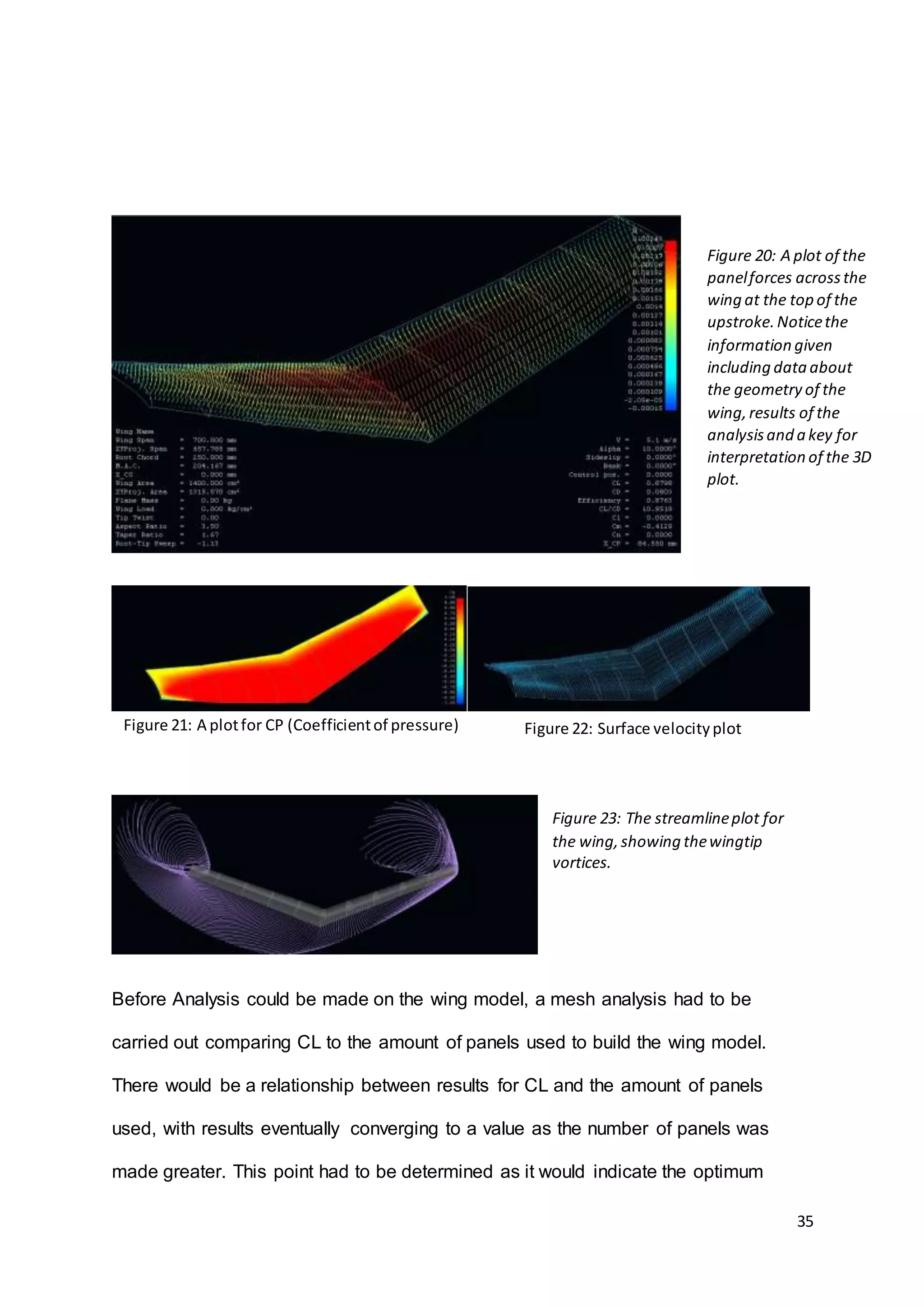
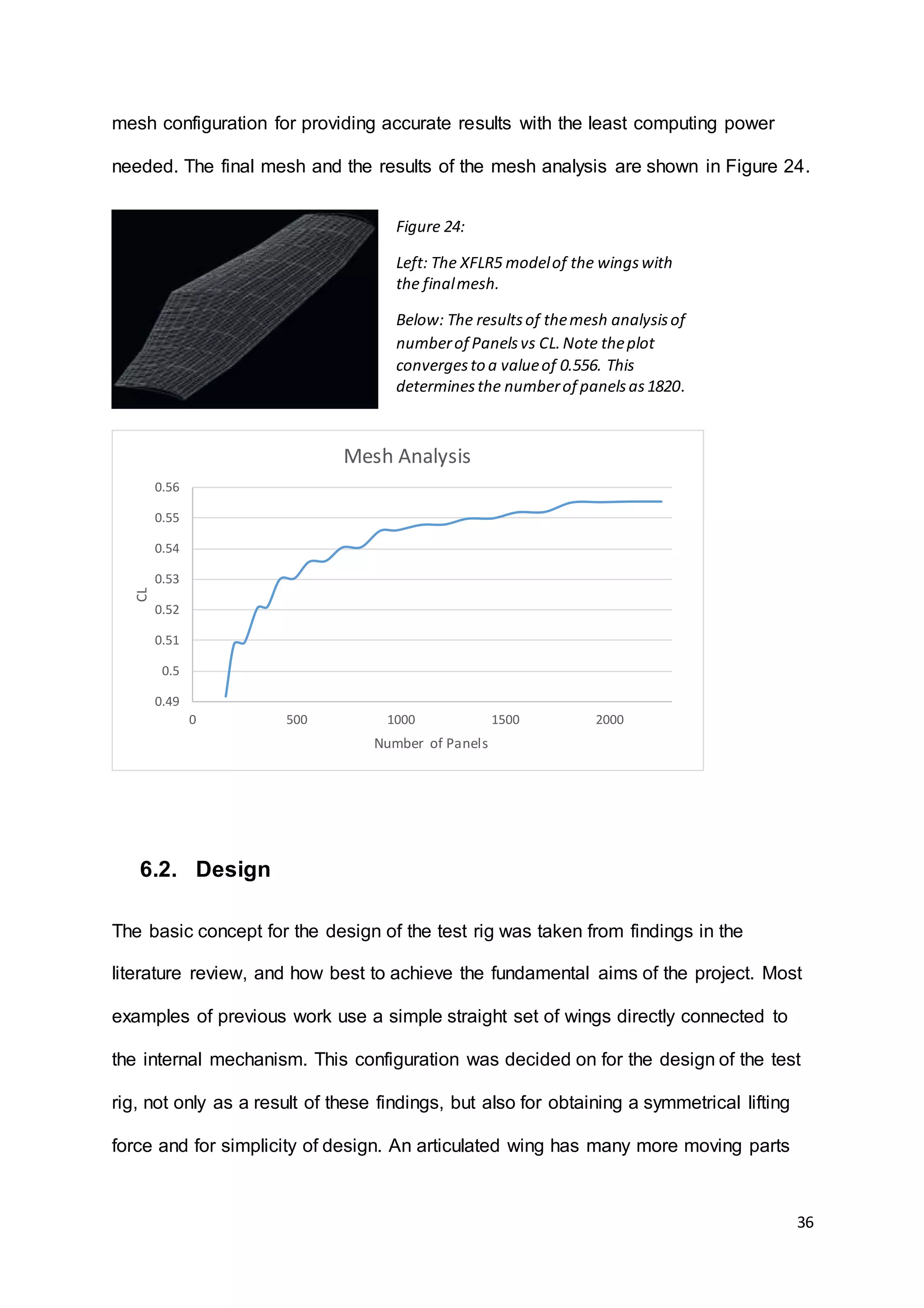
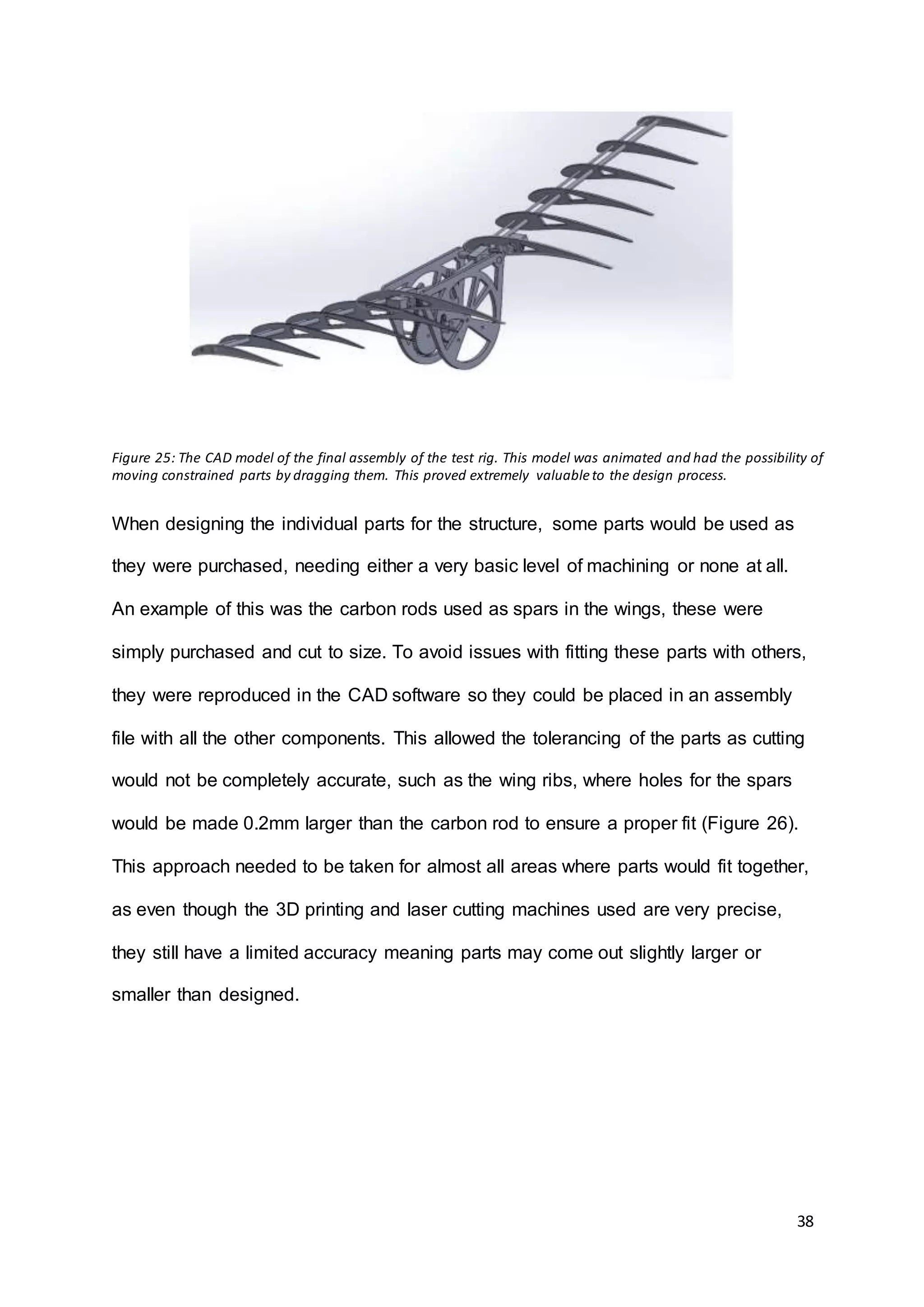
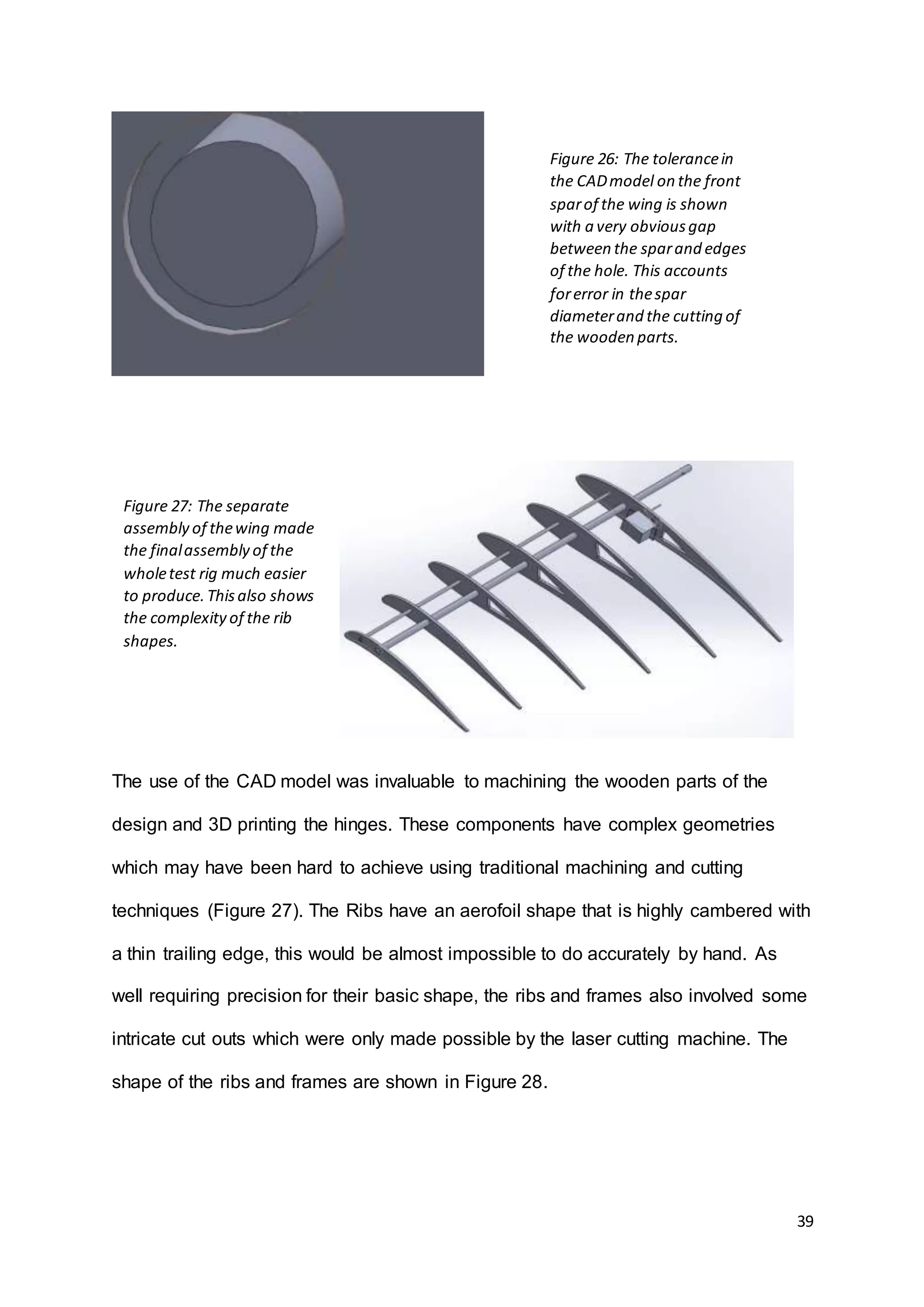
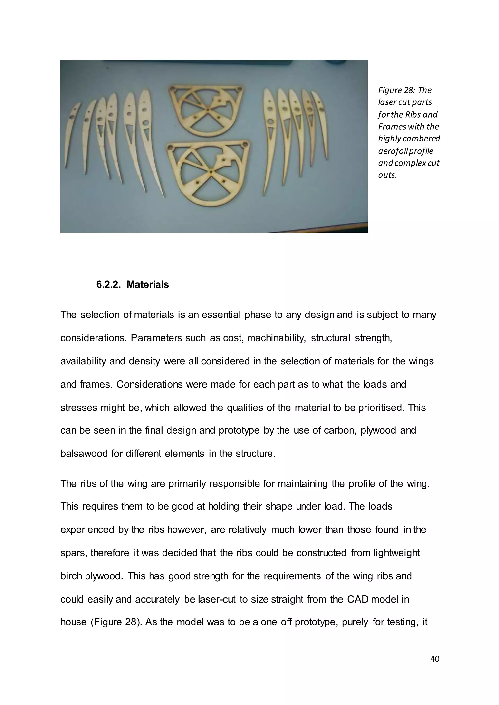
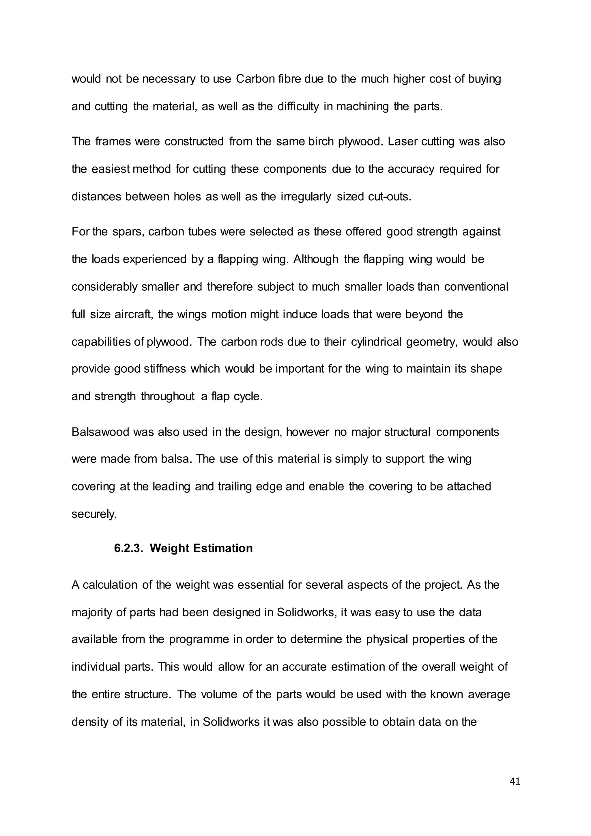
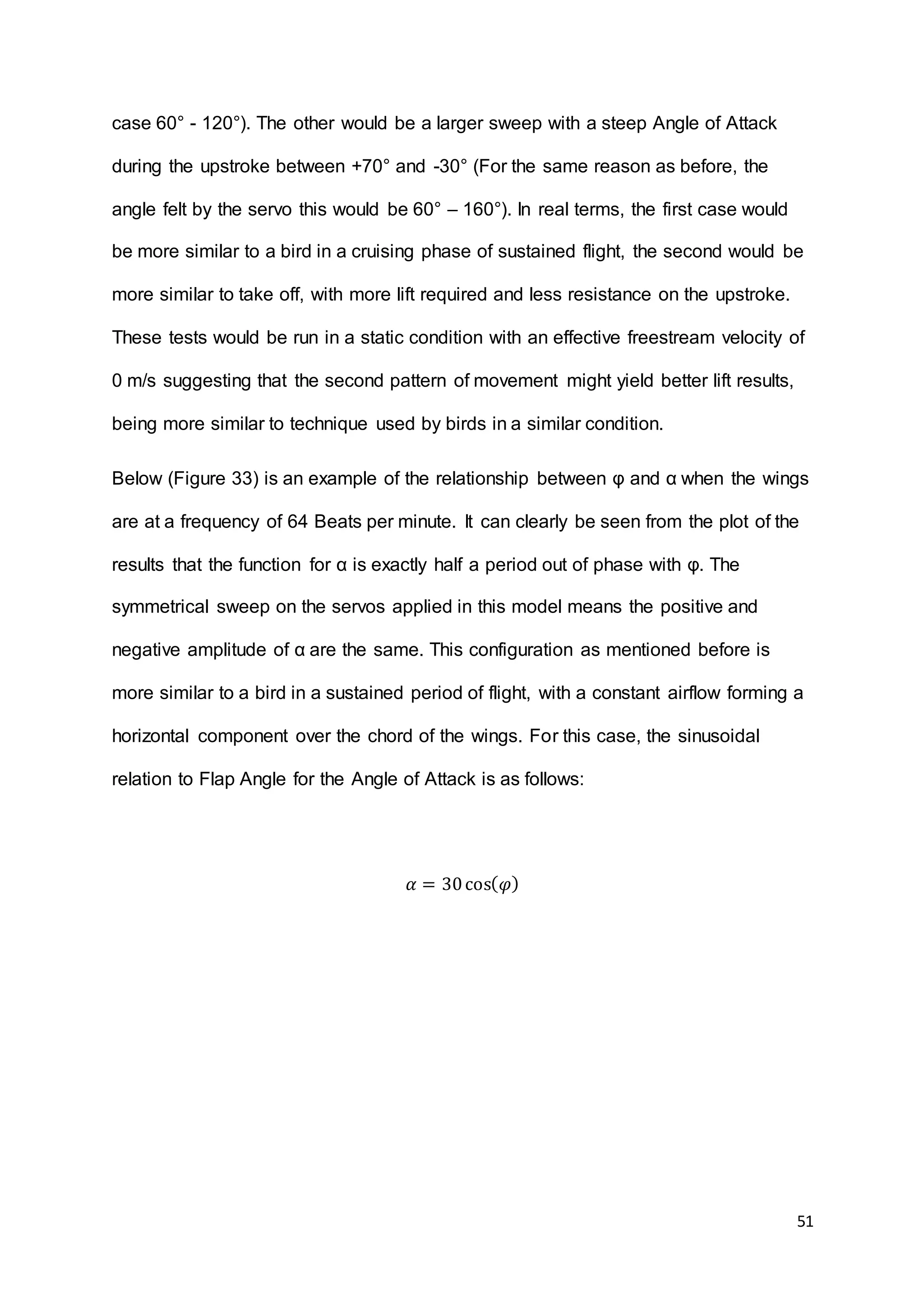
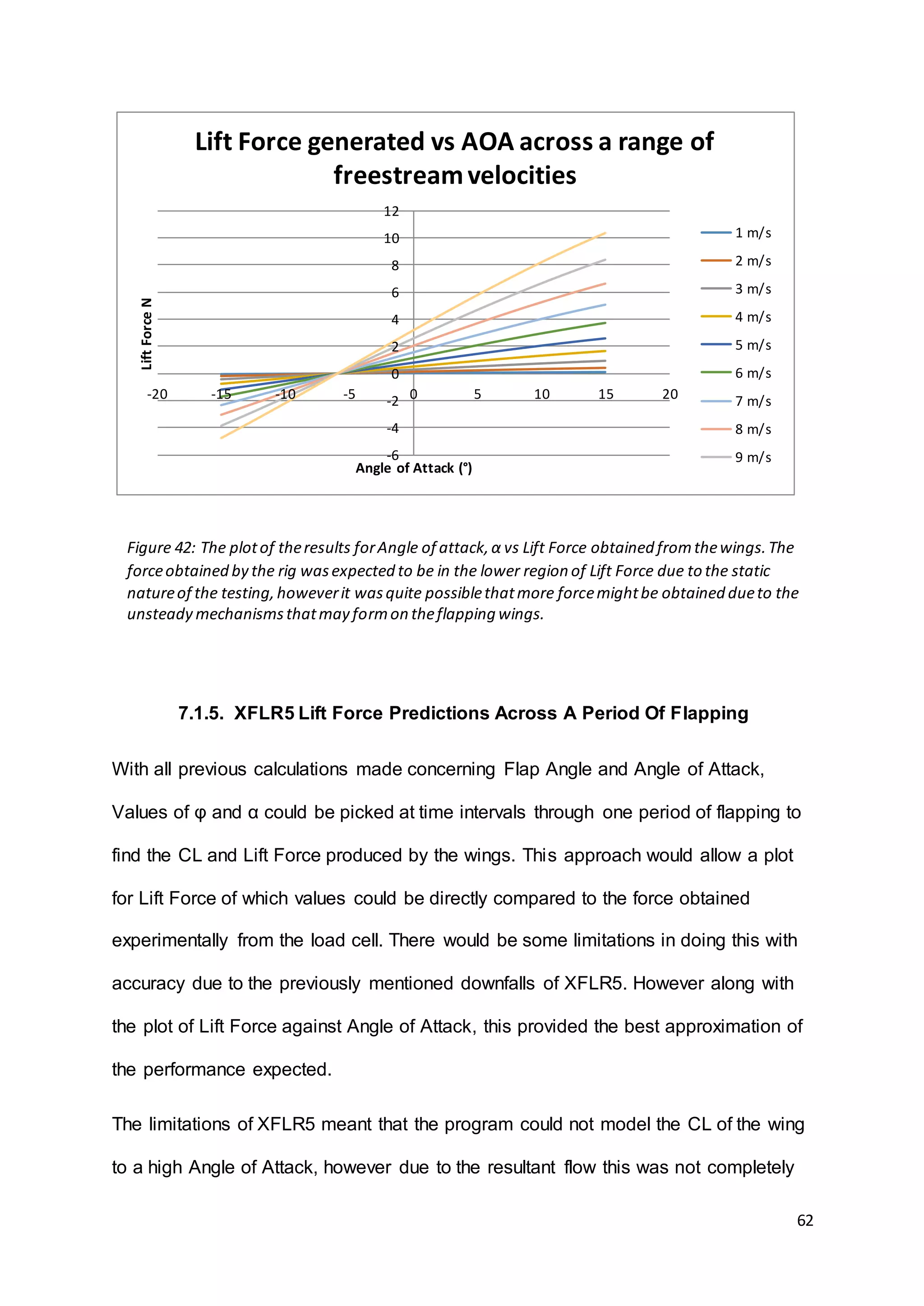
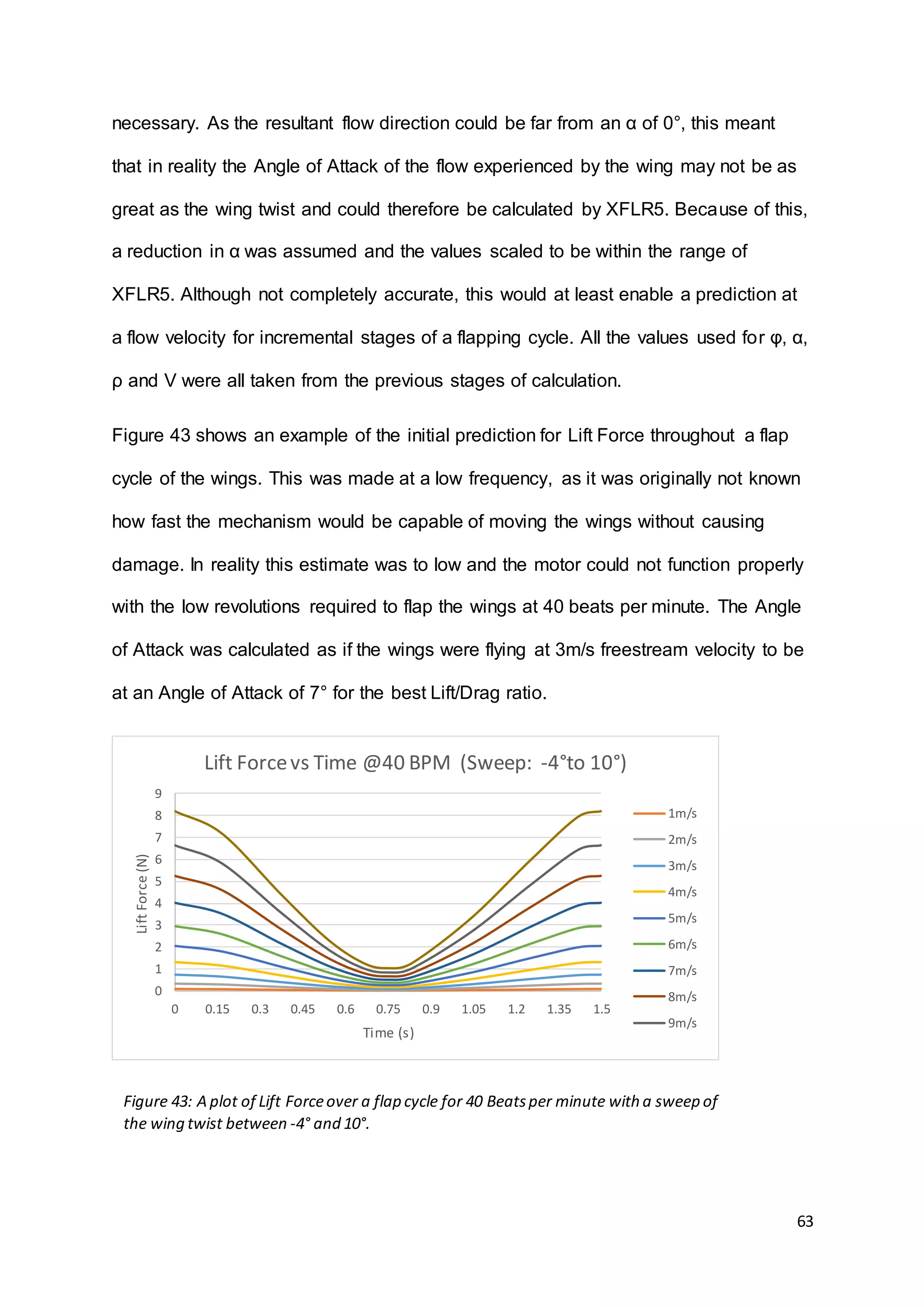
This document summarizes the design and results of a test rig to measure lift force generated by flapping wings. Numerical modeling was used to predict lift values based on wing geometry and motion parameters like frequency and angle of attack. An experimental test rig was designed and built with servo motors in the wings to control twisting instead of relying on flexibility. Force measurements from the rig were taken using a load cell as frequency and angle of attack were varied. Results showed that increasing frequency and angle of attack both increased lift force as expected based on the numerical predictions. The document provides context on bio-inspired flight and reviews other flapping wing projects to inform the design of the test rig.

1. 1
Lift Force Determination in Bio-Inspired
Flapping wings
Author: Sam Knight
Aerospace Engineering MSc
Brunel University
Uxbridge
Abstract: This report details the design and construction of a Test rig flor flapping
wings and compares the results measured from its subsequent use against some
predicted values from numerical modelling. The test rig uses Servo motors mounted
in the wings in order to replace the flexibility of natural wings for the twisting of the
wing during operation. The results conclusively show that an increase in the
frequency of flapping not only applies more force within a set period of time, but also
raises the force achieved per wing beat.

2. 2
Contents
Title Page
1. Acknowledgements 4
2. Notation 5
3. Abbreviations 6
4. Introduction
4.1. Context
4.2. Objectives
4.3. Limitations
4.4. Summary of Methods
7
7
8
9
9
5. Literature Review
5.1. Notable Projects
5.1.1. Festo Smartbird
5.1.2. Clear Flight Solutions: Robirds
5.2. Bird Wing Profiles
5.3. Bird Wing Anatomy
5.4. Models For Flapping Wings
5.4.1. Leading Edge Vortex (LEV)
5.4.2. Rapid Pitch Up
5.4.3. Wake Capture
5.4.4. Clap And Fling Mechanism
5.5. Useful Equations
5.6. Flexibility In Flapping Wings
11
11
11
12
13
14
15
15
16
16
16
17
19
6. Chapter 1: Methods And Design
6.1. Numerical Modelling
6.1.1. Aerofoil Selection
6.1.2. Determining Reynolds Number Of The Flow Regime
6.1.3. Predictions Of Flow Velocity Induced By Flapping
6.1.4. Equations Of Wing Flapping Motion
6.1.5. XFLR5 Analysis
6.2. Design
6.2.1. CAD Modelling
6.2.2. Materials
6.2.3. Weight Estimation
6.2.4. Control
6.2.5. Electronics
6.2.6. Measurement Of Results
20
20
20
23
25
29
32
36
37
40
41
44
46
48
7. Chapter 2: Results
7.1. Results Of Numerical Analysis
7.1.1. Theoretical Relationship of Flap Angle and α
7.1.2. Component Flow Analysis
7.1.3. Lift Predictions Using Calculated CL Values
7.1.4. Lift Force Predictions For The wing Using XFLR5
50
50
50
57
58
60
62

3. 3
7.1.5. XFLR5 Lift Force Predictions Across A Period Of
Flapping
7.2. Experimental Results
7.2.1. Symmetrical Positive And Negative α Study With
Increasing Frequency
7.2.2. High Positive α Study With Increasing Frequency
7.2.3. Increasing α Sweep Study At Constant Frequency
65
67
69
70
8. Chapter 3: Analysis
8.1. The Design
8.2. Flap Angle, φ And Angle Of Attack, α
8.3. Comparisons Between The Lift Force Calculated And Lift
Force Determined Experimentally
8.4. The Relationship Of Lift Force And Frequency
8.5. The Relationship Of Lift Force And α
74
74
77
78
83
87
9. Conclusion 92
10.References 95
11.Project Management 97
12.Appendix: Dissertation Proposal: Bio-Inspired Flying Machines 99
13.Appendix 103

4. 4
1. Acknowledgements
I would like to thank my tutor Dr Farbod Khoshnoud for the support, help and
inspiration he gave me for this project. His enthusiasm for the project and the subject
area ensured I stayed motivated throughout the whole period of work.
Recognition must also go to my family who were also very supportive of my work
and helped in whichever way they could.
Others who inspired my ideas and solutions as well as helped me with my work such
as the university technicians also must get a large amount of recognition as without
their expertise and knowledge of equipment obtaining the results I needed would
have been far more challenging.

5. 5
2. Notation
 RE – Reynolds Number
 V – Velocity
 𝑉∞ - Freestream Velocity
 𝑉𝑅𝐸𝑆 – Resultant Flow Velocity
 𝑉𝐶𝐺 𝑀𝐴𝑋
– Maximum Wing centre of Gravity Velocity
 𝑉𝐺𝑀𝐴𝑋- Maximum velocity of wing Centre of Gravity
 mph – Miles Per Hour
 m/s – Metres per Second
 cm/s – Centimetres per second
 ω 𝑤 – Wing Angular Velocity
 ω 𝐺 – Gear Angular Velocity
 𝛼 𝑅𝐸𝑆 – Angle of Attack of the Resultant Flow
 ° - Degrees (Angle)
 kg – Kilograms
 g – Grams
 m – Metres
 cm – Centimetres
 mm – Millimetres
 l – Chord
 𝑥̇ – Rate of Change of Distance
 𝑟𝐺 - Gear Radius
 𝑟ℎ𝑖𝑛𝑔𝑒 – The Inboard Length of the Spar from push rod linkage to Hinge
 𝑟𝐶𝐺 – Distance from the Hinge to the wing Centre of Gravity
 𝐴 𝑊 – Wing Surface Area
 s - Second
 𝑓- Frequency
 T - Period
 CL – Coefficient of Lift
 CD – Coefficient of Drag
 α – Angle of Attack
 φ – Flap Angle
 𝜑̇ – Rate of Change of Flap Angle
 ρ – Air Density (1.225 kg/m^3
 μ – Dynamic Viscosity
 ν – Kinematic Viscosity (1.5*10^-5 kgm^2/s)
 𝐿 – Lift Force
 N - Newton

6. 6
3. Abbreviations
 MAV – Micro Air Vehicle
 LEV – Leading Edge Vortex
 CAD – Computer Aided Design
 ESC – Electronic Speed Controller
 BPM - Beats per Minute
 CG – Centre of Gravity

7. 7
4. Introduction
4.1. Context
Humans have been taking inspiration for the design of aerospace vehicles from
nature centuries before the wright brothers made their first flight in 1903. However
until quite recently, efforts to fly as a bird or insect under the power of flapping wings
have been largely unsuccessful. Within the past two decades or so, new
manufacturing techniques, leaps forward in control and electronics, and experience
gained using strong lightweight materials have brought about some successful
examples of flapping wing flight. Such aircraft are often referred to as MAV’s (Micro
air vehicles) were the aircraft is usually the size of a bird or remote control plane.
Commercially, even though unsuitable for manned flight there is a large amount of
scope for a Flapping wing MAV, though methods used for their flight and control are
still much under development with a variety of theories on how a successful project
would be best achieved.
A successful flapping wing MAV vehicle has scope to be sold and operated in a
variety of sectors. These span through military, intelligence, agricultural, surveying
and search and rescue organisations who all have use for Bio-Inspired air vehicles.
The attraction for such a vehicle comes from its similarities to birds and how they
overcome some fundamental flaws with current aircraft and helicopter systems. A
birds control through flapping wings allows them to be very manoeuvrable and
access areas that an aircraft could not, such as flying in tight spaces within rock
formations, a particular advantage in the search and rescue application. However, a
bird is also able to cover a lot of ground in a short space of time which a MAV

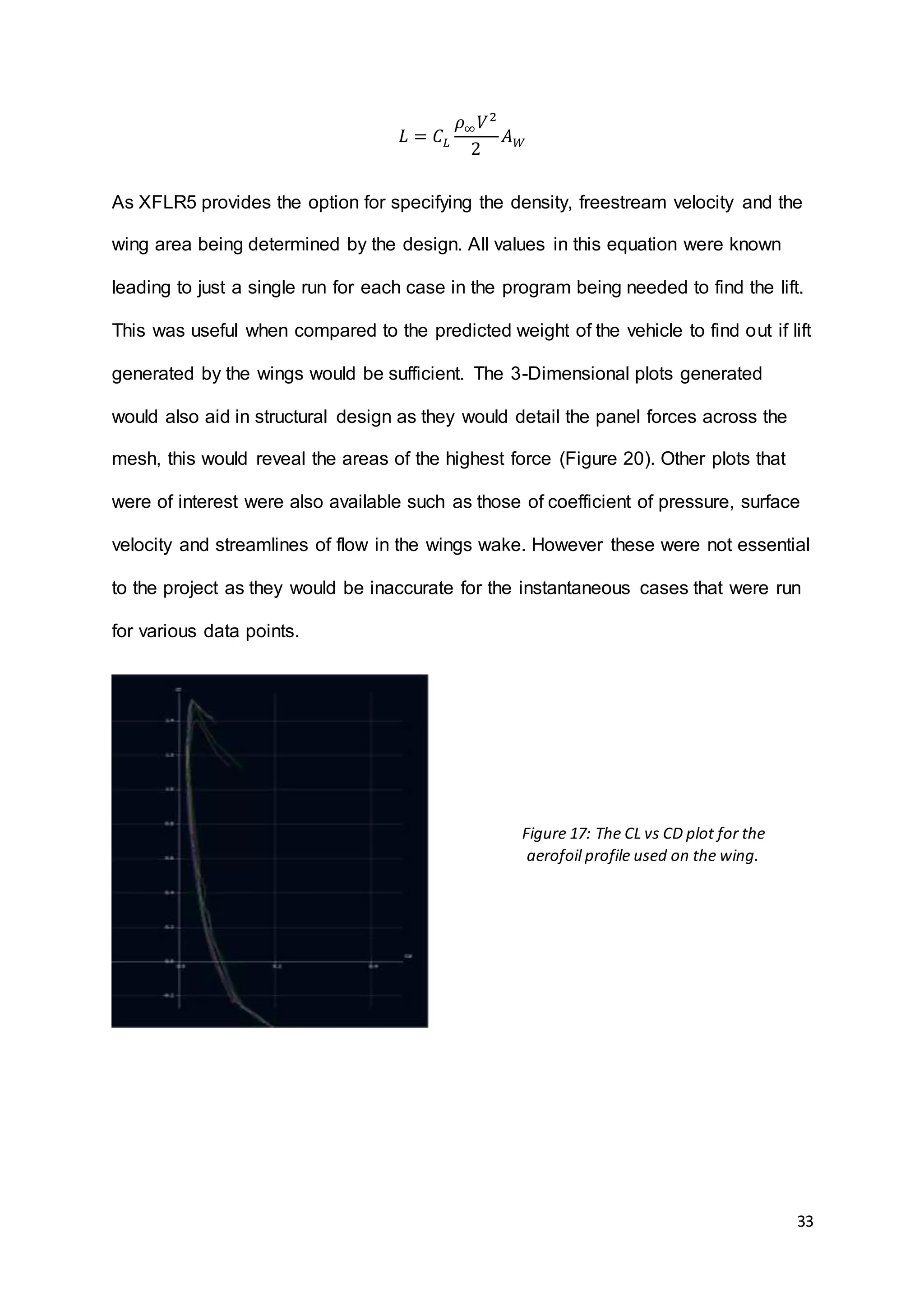
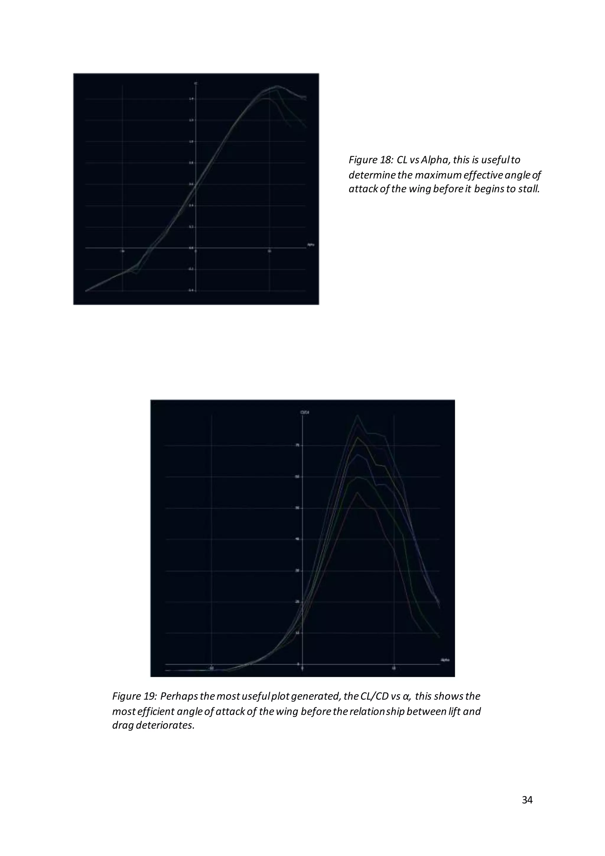
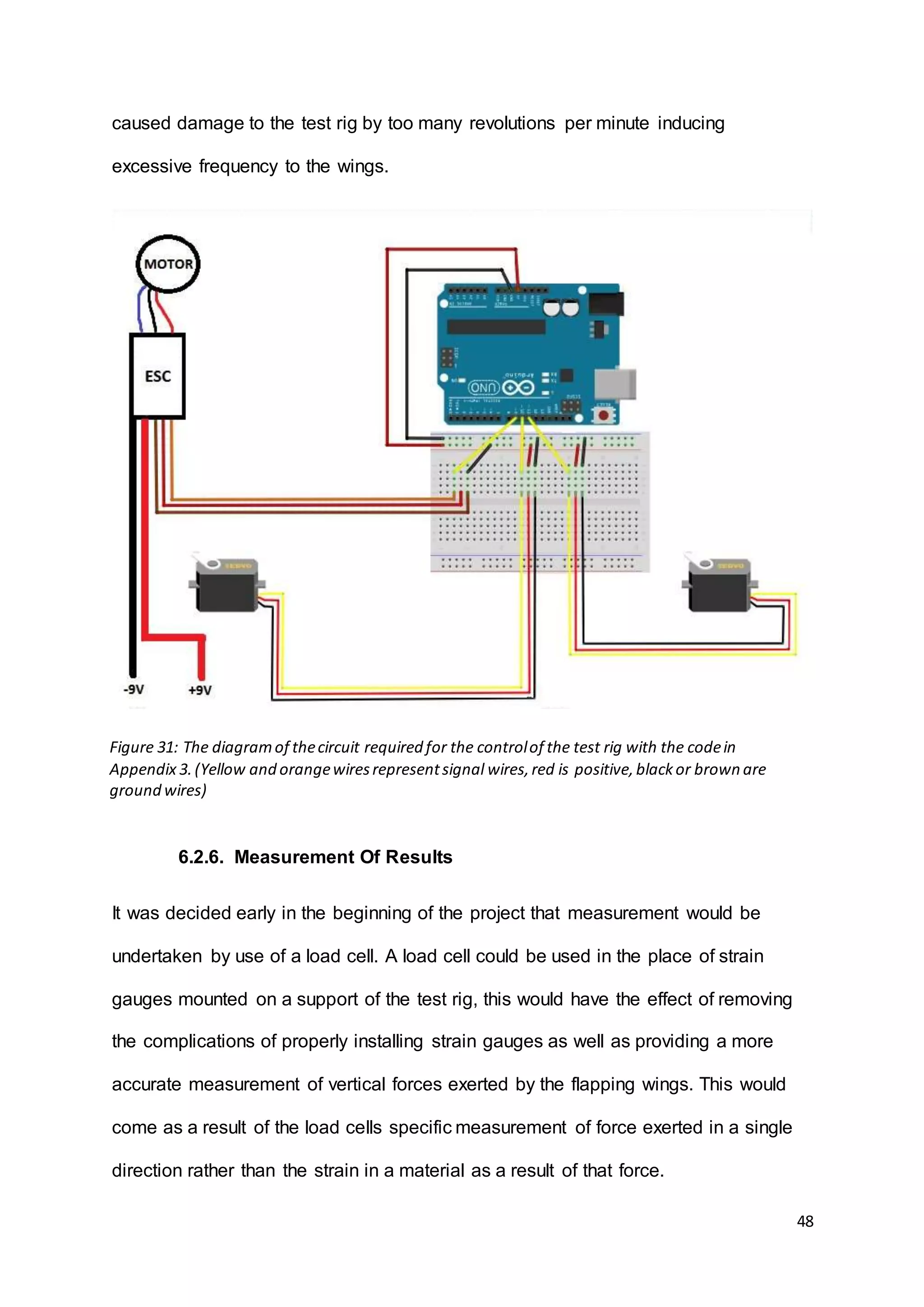
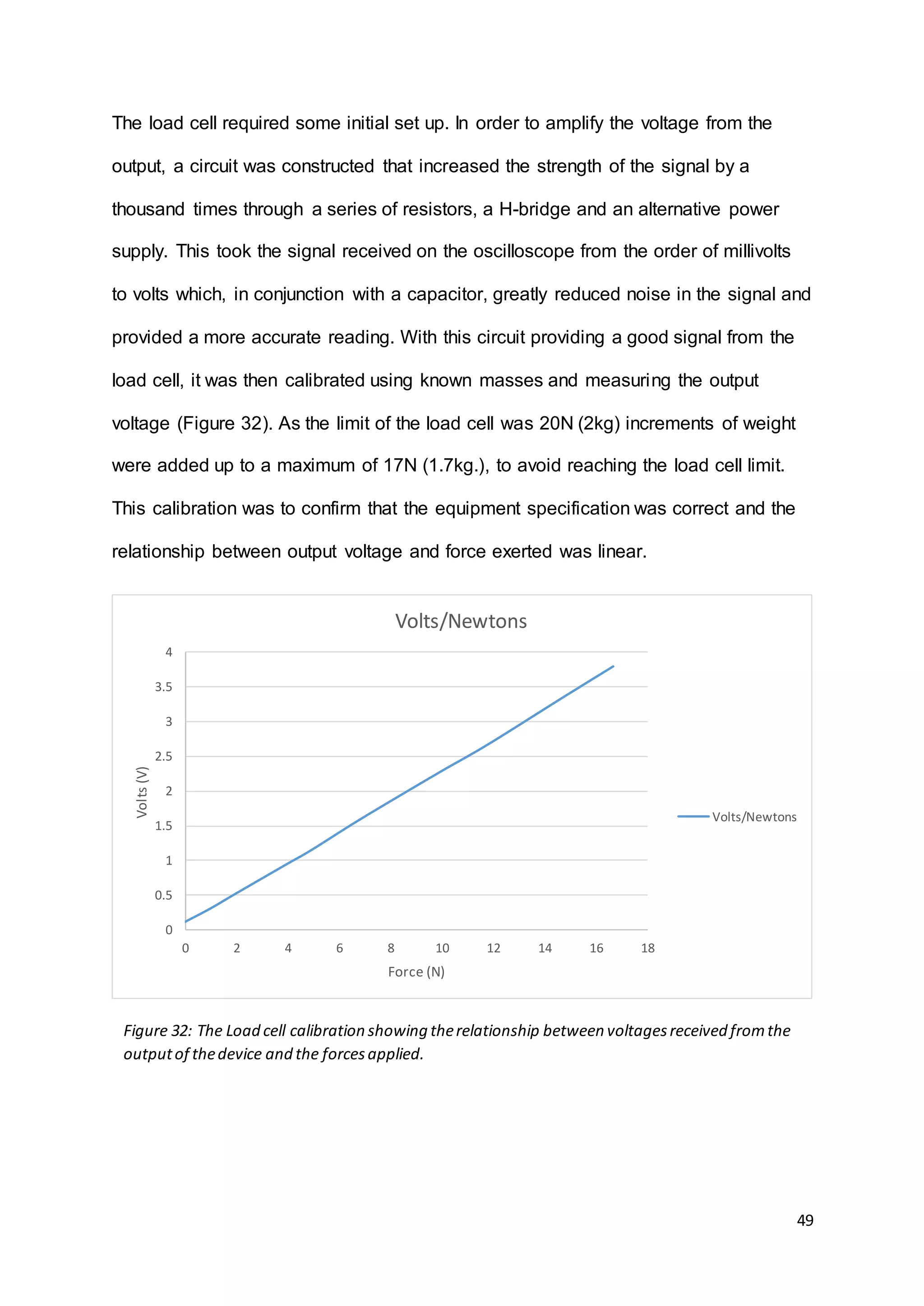
8. 8
helicopter system could not. It is this versatility which makes a viable Bio-Inspired
flapping wing vehicle a desirable asset for many applications.
4.2. Objectives
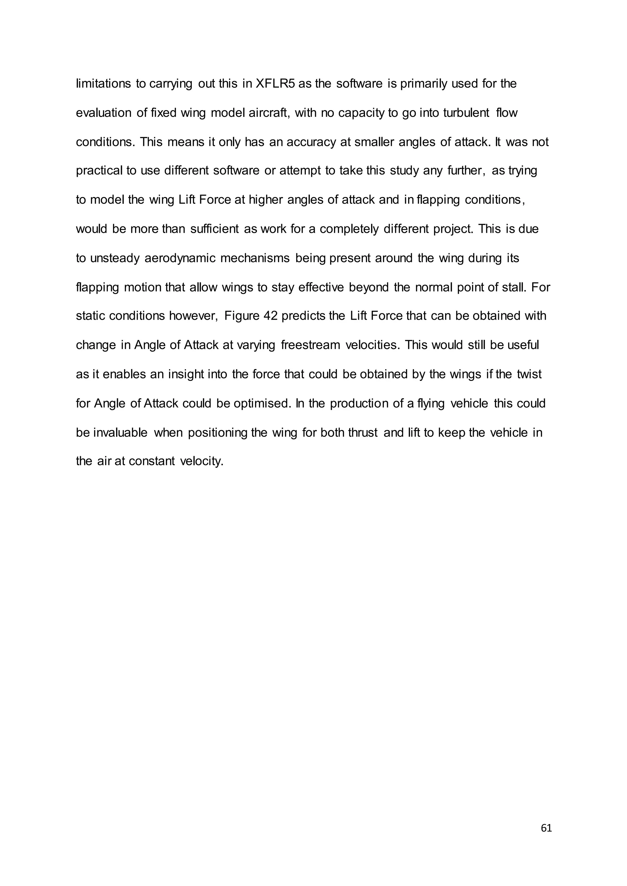
The main focus of the project will be the measurement of Lift Force exerted by a pair
of flapping wings. Where natural examples use passive wing flexibility [1], which
provides the necessary characteristics to a birds wings relative to the conditions they
experience. The design of the test rig however will seek to use servo motors in built
to the wing to replace the need for wing flexibility and its complex design problems.
As much as possible, inspiration will be taken from biological examples with regard
to the shape of aerofoil used and wing geometry. Analysis of the wings will be
carried out numerically to obtain predicted values for Lift Force in the planned
studies for the increase in frequency and stroke Angle of Attack (α).
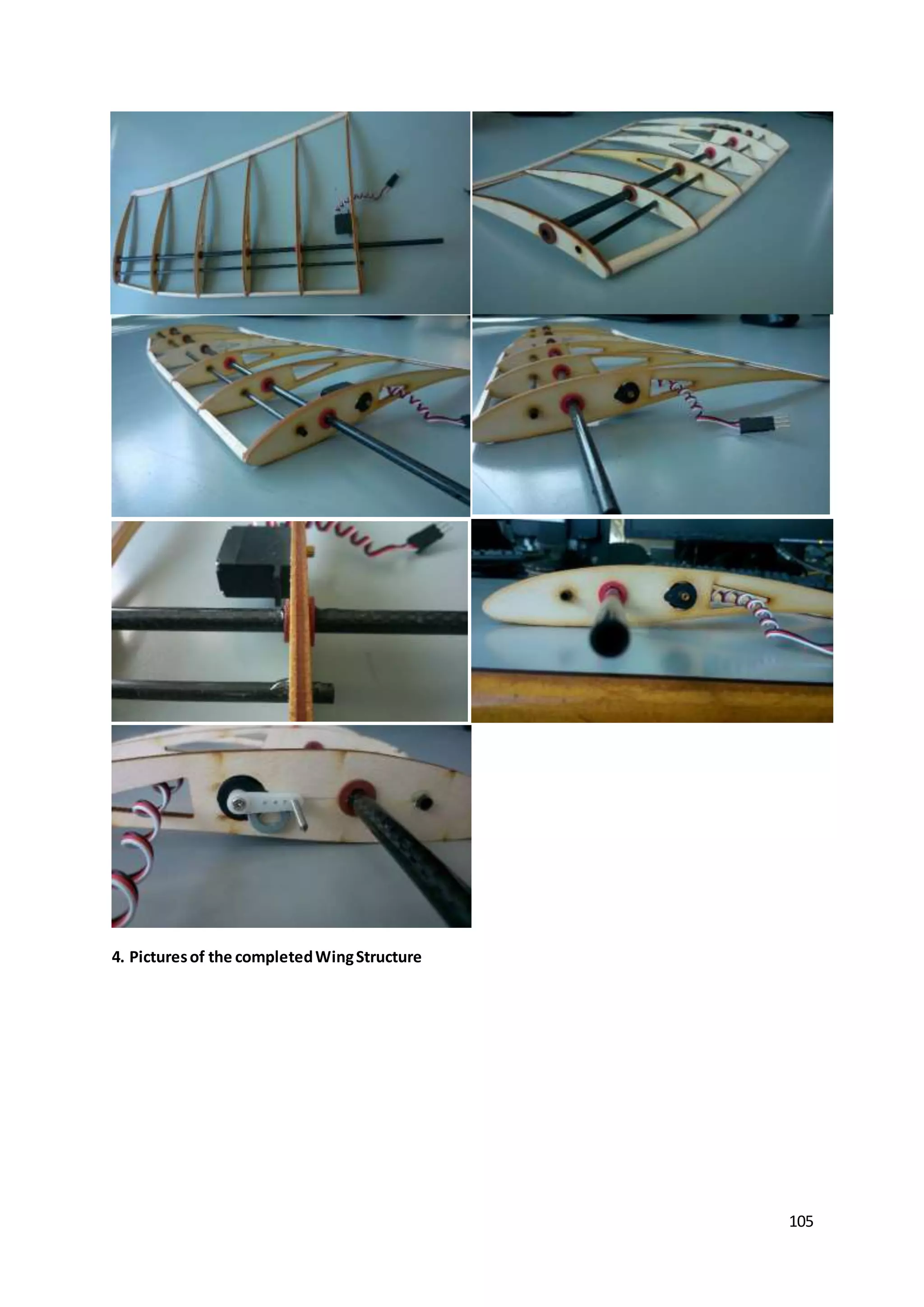
With results predicted for the test rig, the design will then be finalised and
constructed. This will seek to use, if possible the same material that would be used
should the design be applied to a flight vehicle. The design of the test rig will
incorporate a pair of wings each with an internally mounted servo in order to twist the
wing, as well as a frame which will hold the wings, motor and mechanism necessary
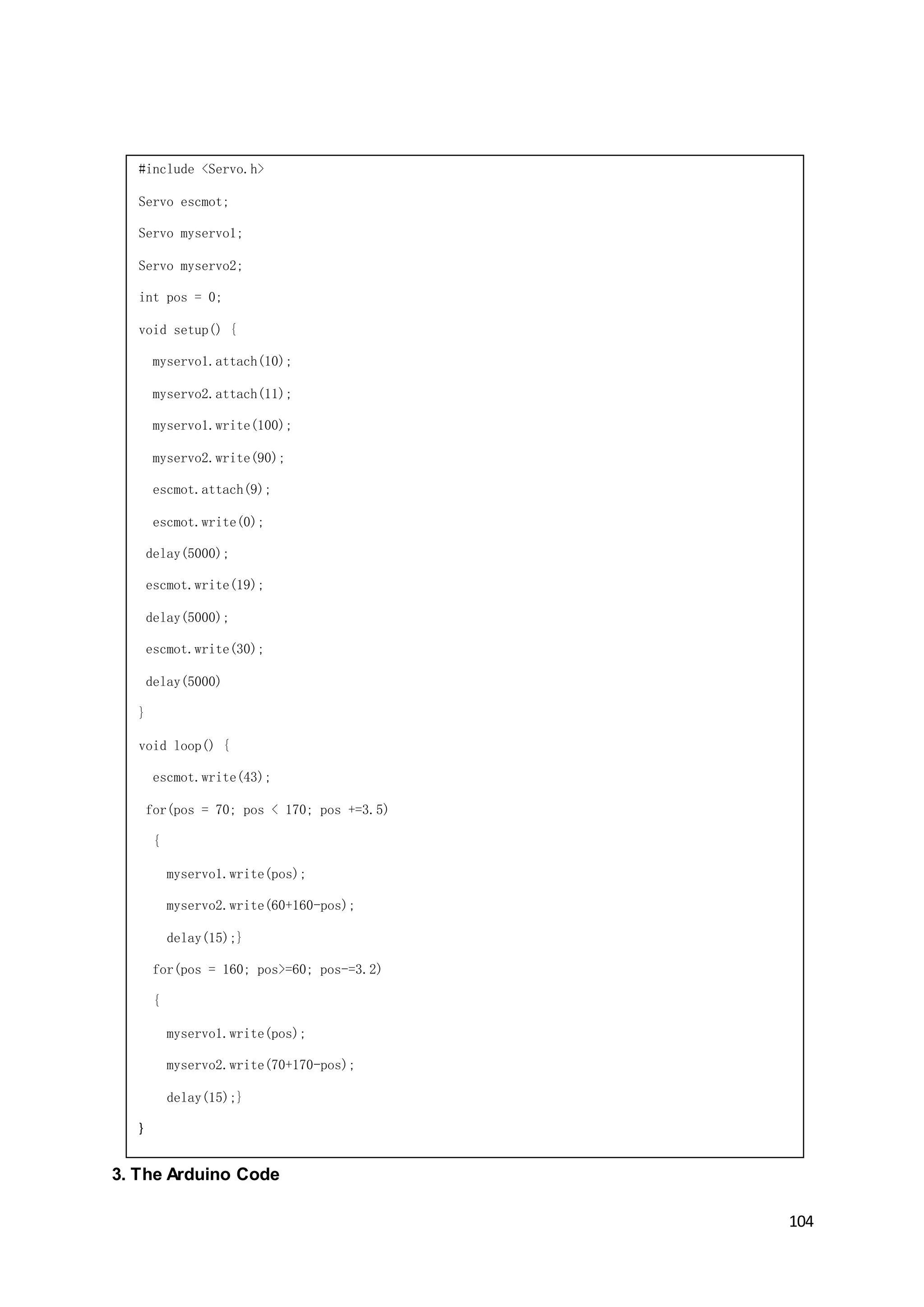
for their flapping motion. Control will be achieved with the use of an Arduino board,
this was selected due to the ease of controlling servos and a brushless motor.
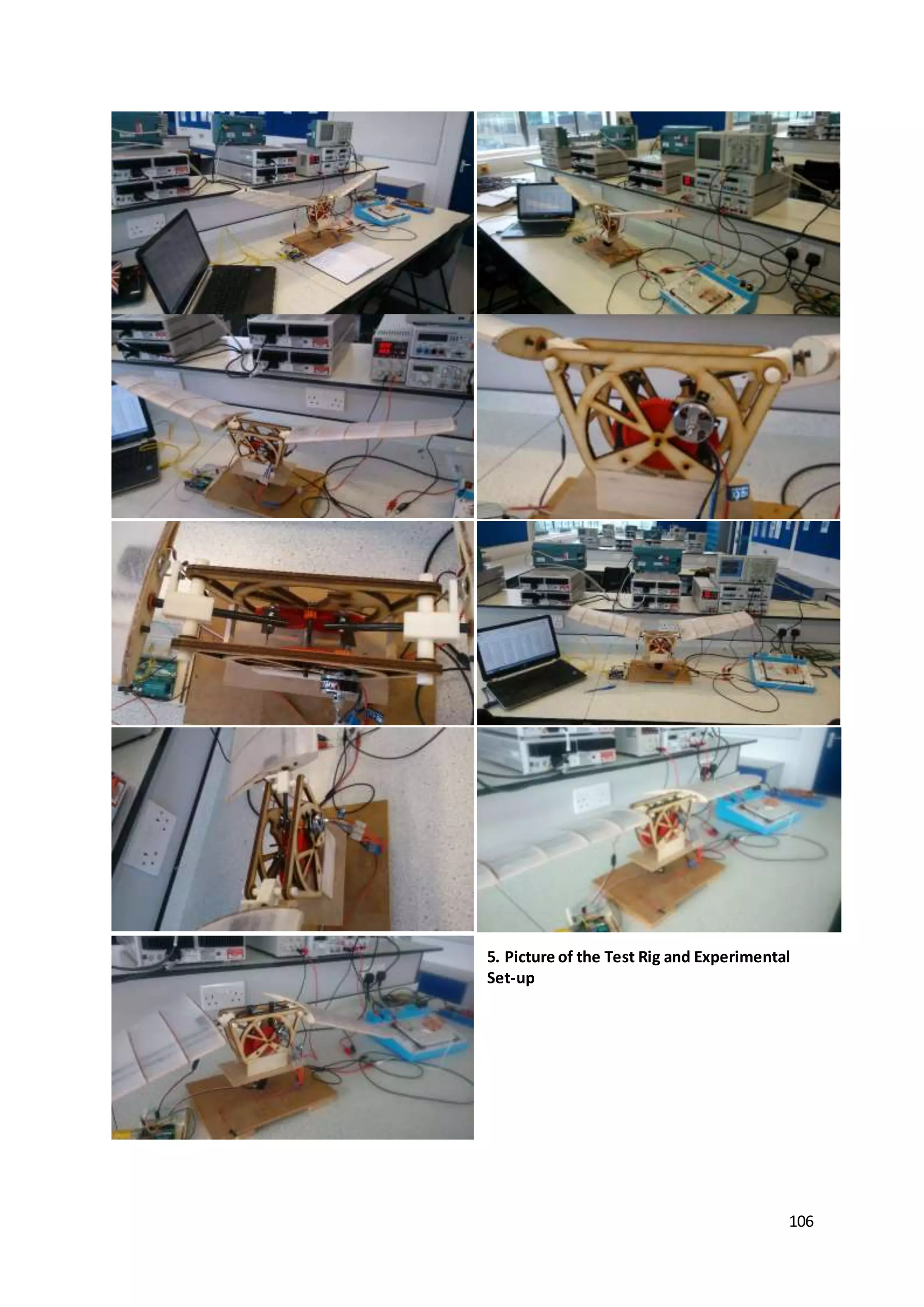
The measurement of the results experimentally will be achieved by the use of a load
cell. This decision was made through the experience of the inadequacy of strain
gauges mounted on a stand holding the test rig. This would allow force to be
measured in a single direction with the direct output relationship to force being
extremely attractive with regard to the processing time of results. The load cell would

9. 9
be mounted between a base plate clamped to a desk, and the test rig, in a vertical
position to exclusively measure the forces created in a vertical direction. Once the
measurements had been taken these would then be compared to those calculated
and the differences and similarities discussed.
4.3. Limitations
As there is a timescale for the project, this will be a large factor into completing the
work as planned. Provisions have been made in order to ensure that the project
remains active throughout its duration, and delay’s due to the delivery and machining
of parts will not be responsible for the projects failure. For ease of construction, the
test rig must be built to have a wing span of around 70cm. Although this allows or
easier construction and sourcing of parts, there are drawbacks to the relatively large
wingspan. All tests will have to be carried out in static airflow with the test rig being
too large for the wind tunnels available. This may cause some difference between
the predicted and measured results due to the inability to calculate values of Lift
Force with a velocity of 0m/s. Lastly, a potential limitation in the materials used could
be the difficulty of machining carbon fibre. This would be the material of choice for
the test rig structure, however it is costly to machine and requires specialised tooling
which cannot be provided in house. In the event of this not being possible, the
carbon fibre parts can be machined from plywood.
4.4. Summaryof Methods
The numerical analysis will be challenging, due to the 3-dimensional nature of a
flapping wing problem. This will be done using two approaches, the first will be in
XFLR5. This provides a visual representation of the design wing which will aid in the
design of the structure for the test rig, allowing dimensions to be clearly seen

10. 10
alongside the wing geometry. XFLR5 can then analyse the wing using data from an
aerofoil analysis, which is also conducted in the software, to produce values for CL.
The second method of obtaining Lift Force will be using equations and methods used
in previous work and applying these to the predicted changes in the parameters of
Flap Angle (φ) and α.
The measurement of experimental data will be done over two studies. The first will
be the increase in frequency over two different Angle of Attack configurations. One
with a symmetrical movement between identical values of positive and negative α.
The other with a high positive Angle of Attack with the aim of creating a more
efficient pattern of movement. The second study will be into the Angle of Attack
achieved at the peak velocity point of the downstroke, this will aim to determine if Lift
Force is increased with a larger negative α or to find its optimal value. The result of
each set case for testing will be analysed using the same method as used by Sane
S.P. (2001) [2] where multiple wing strokes are taken and averaged into a dataset for
a single wing stroke.

11. 11
5. Literature Review
5.1. Notable Projects
5.1.1. Festo Smartbird
Perhaps the most successful attempt at recreating bird flight, this example uses a
lightweight carbon structure, weighing only 450grams with a wingspan of nearly
2meters. A high gearing ratio between the motor and the mechanism ensures that a
relatively small motor can drive its wings. The key feature of the Smartbird is the
active torsion designed into its wings. This consists of a servo mounted towards the
wing tip, on the outer most wing rib. This is connected to a microcontroller to
calculate the input from information drawn from an array of sensors for acceleration,
torsional force on the hand wing, and motor position. Data acquired from testing,
provides the relevant information in order to position the hand wings to twist into an
optimised position for the current flight conditions and phase of wing motion [3]. This
approach brings this design closer to its natural inspiration than any other design;
with it not only mechanically replicating the movement and motion of the bird’s
skeleton and muscles, but also replicating the bird’s sensory system by the various
on-board sensors. Festo has also undertaken other projects with flapping wings
drawing inspiration from dragonflies and butterflies in some of its other notable
Bionic Learning Network projects, known as the BionicOpter [4] and
eMotionButerflies [5].

12. 12
5.1.2. Clear Flight Solutions: Robirds
Designed as a deterrent for nuisance birds around airports, waste and agricultural
sites [8], their manufacturer claims significant reductions in numbers of smaller birds
from repeated use in a given area [9]. However, they are not currently commercially
available and are still undergoing development. Unlike the Smartbird, the wings are
not articulated and do not contain servos to optimise twisting. They are however of a
flexible foam construction. A front and rear spar move to twist the chord of the wing
which provides lift and thrust. With regard to control, the Robirds do not have the
same aerodynamic turning effects with the tail and head moving together, however
enough manoeuvrability is still achieved for operation within an outdoor space.
Currently two types are being developed to replicate a peregrine falcon and an
eagle, which are still in the testing phase with an aim to make their flight completely
autonomous with an autopilot system. Perhaps not as technologically advanced as
the Smartbird, the Robirds do however have the speed to match their natural
equivalents, with a manufacturer’s claim of a 50mph top speed in the Falcon model
[10].
Figure 1: The Festo Smart bird [6] Figure 2: A CAD imageof the
Dragonfly inspired BionicOpter[7]

13. 13
5.2. Bird Wing Profiles
Various attempts have been made to model bird wing profiles, however this proves
challenging in practice. A number of approaches have been tried, but due to the
nature of avian wings and their unique flexibility to suit a range of flight profiles, great
effort is required in order to obtain a profile for even one flight state. One initial
approach was to take measurements from museum specimens [11] and treat these
as fixed aerofoils rather than a highly deformable bird wing. However this method is
inaccurate due to the necessary process of preservation. Recently deceased
specimens [12] also experience problems in the uncertainty in what flight conditions
the wing was last set for. Even without these effects, errors would still occur as when
a bird is in flight, its sensory system is constantly optimising the wing through
differing flight stages [13]. Therefore the variables the wing experienced most
recently would be unidentifiable. Through this, the optimum method utilised is to
measure the wing whilst in flight. One such method by the Oxford department of
Zoology used a trained bird and photogrammetric techniques in order to pin
coordinates to points on the wing to model the inner surface. This was done by
setting up a series of six cameras around a known control volume containing a perch
on which the trained steppe eagle would land [14]. This meant measurements were
taken in a rapid pitch up manoeuvre from a shallow glide into a stall to land. Similar
work to this had already been undertaken, however this involved smaller birds in
Figure 3: The Clear flight solutions
Falcon model.The wing shapeplays
a large partin its successasa bird
deterrentwhich when flapping looks
similar to the real bird. [8]

14. 14
wind tunnels with sparrow [15] and starling [16] test subjects. The use of smaller
birds provides little insight into Reynolds number regimes that would be experienced
by MAV’s built with current technology, as it is unlikely that a smaller bird species
could be replicated.
5.3. Bird Wing Anatomy
Although in many ways very different, the avian wing demonstrates numerous
similarities to the human arm [17]. Both in bone structure and the associated
muscles to drive movement. There are recognisable shoulder, arm and hand
sections to the bone structure, with the hand wing forming the significantly larger
area towards the tip of the wing containing the primaries [17] (primary feather group-
the largest feathers on the wing). The feathers attached to the arm wing are known
as the secondaries [17]. Unlike in a human arm, the arm wing in a bird accounts for
less than half of the total wing span. Other feather groups are known as the coverts
and the scapulars, with the coverts forming the feather covering of the leading edge
and the centre of the wing surface. Other notable similarities between birds and
humans is the presence of pectoral muscles used for flapping the wings down [18],
humans have similar muscles in the chest used to move their arms forward and
together.
Figure 4: The profiles thatresulted
fromthe photogrammetricstudy
undertaken by theOxford department
of zoology of a Malesteppe eaglein a
high pitch up manoeuvre.[14]

15. 15
5.4. Models For Flapping Wings
In order to design an optimised flapping wing MAV with the flight characteristics of a
real bird, the problem has to be numerically understood. Considerable work has
been done on the angle of attack, flap angle, and wing beat frequency, as well as
four unsteady mechanisms that frequently occur, and various other variables
associated with not only airflow but also a constant movement of the wings. Four
unsteady mechanisms cited frequently in literature are leading edge vortices, rapid
pitch up, wake capture and clap and fling [20]. These mechanisms are typical of
problems faced as they clearly aid in lift production in insects and birds but are
difficult to predict for variations with current methods of analysis. In further detail,
these models are described as follows:
5.4.1. Leading Edge vortex (LEV)
A flow of air created around the front of the wing which rolls over the leading edge
during the downstroke. The low pressure at the centre of the vortex creates a suction
force that attaches it to the wing during the stroke and increases the possible angle
of attack before stall is induced. This creates higher lift than is normally obtainable by
the same wing and enhances the performance of the wing over its capabilities in
Figure 5: the labelled arrangement
of featherson a bird wing. [19]

16. 16
steady state flow. The vortex has been found by studies to be conical in shape,
having a smaller radius towards the root of the wing and much larger diameter at the
wing tip. This is due to the increases in the wings tangential flow velocity along the
span. This mechanism has been identified as the most significant in flapping wing
flight to increase the lift, however observations vary as to the LEV’s behaviour on
different wings. In some cases it is seen to be permanently attached, whereas in
other cases it sheds and reforms with each beat.
5.4.2. Rapid Pitch Up
A quick rotation at the end of each stroke, where the wing moves from a low to high
angle of attack, generating much higher lift coefficients than the steady state stall
value [20].
5.4.3. Wake Capture
Occurs as a wing travels through the wake it created on a previous wingbeat.
Research has shown peaks in aerodynamic force when the wake of a previous wing
beat is captured with correct phasing and twist of the wing [20].
5.4.4. Clap And Fling Mechanism
This refers to the way the set of wings are moved during the wingbeat. The majority
of birds do not use this type of motion in normal flight, however some, such as the
hummingbird could be described to use a clap and fling motion. More applicable to
insect flight, this model for wing movement describes the upward motion (the clap),
where the wing leading edges are clapped together at the end of the upstroke. The
downstroke consists of the leading edges moving apart whilst the trailing edge
remains stationary, therefore the wing rotates around the trailing edge. This is known
as the ‘fling’ [19].

17. 17
5.5. Useful Equations
For the Numerical Analysis of the project there are some papers for work previously done
that provide good methods and equations that could be applied. These studies carried out
are notably those by Whitney J.P (2001) [22], and Dickinson M.H. (1999) [23]. Both provide
good relationships to be followed and good approximations of CL and CD to be applied to
flapping wings.
The Study by Whitney [22] focuses on conceptual design of MAV’s with no practical work
undertaken. A large focus of the paper is on the hovering energetics and predicting the flight
performance such as the range and speed of the vehicle. However, of interest to this project
is the work undertaken to predict the damping force and the relationship produced between
φ and α (Figure 7). This would be useful to predict the timing of the parameters of the test rig
wings and apply further calculations to obtain the wings lifting force as a function of the
theoretical angle of attack.
Figure 6: The clap and fling
mechanism,herethe diagramsare
shown asif looking fromabovethe
insect/ bird and the circular ends
representthe leading edge of the
aerofoil.[21]

18. 18
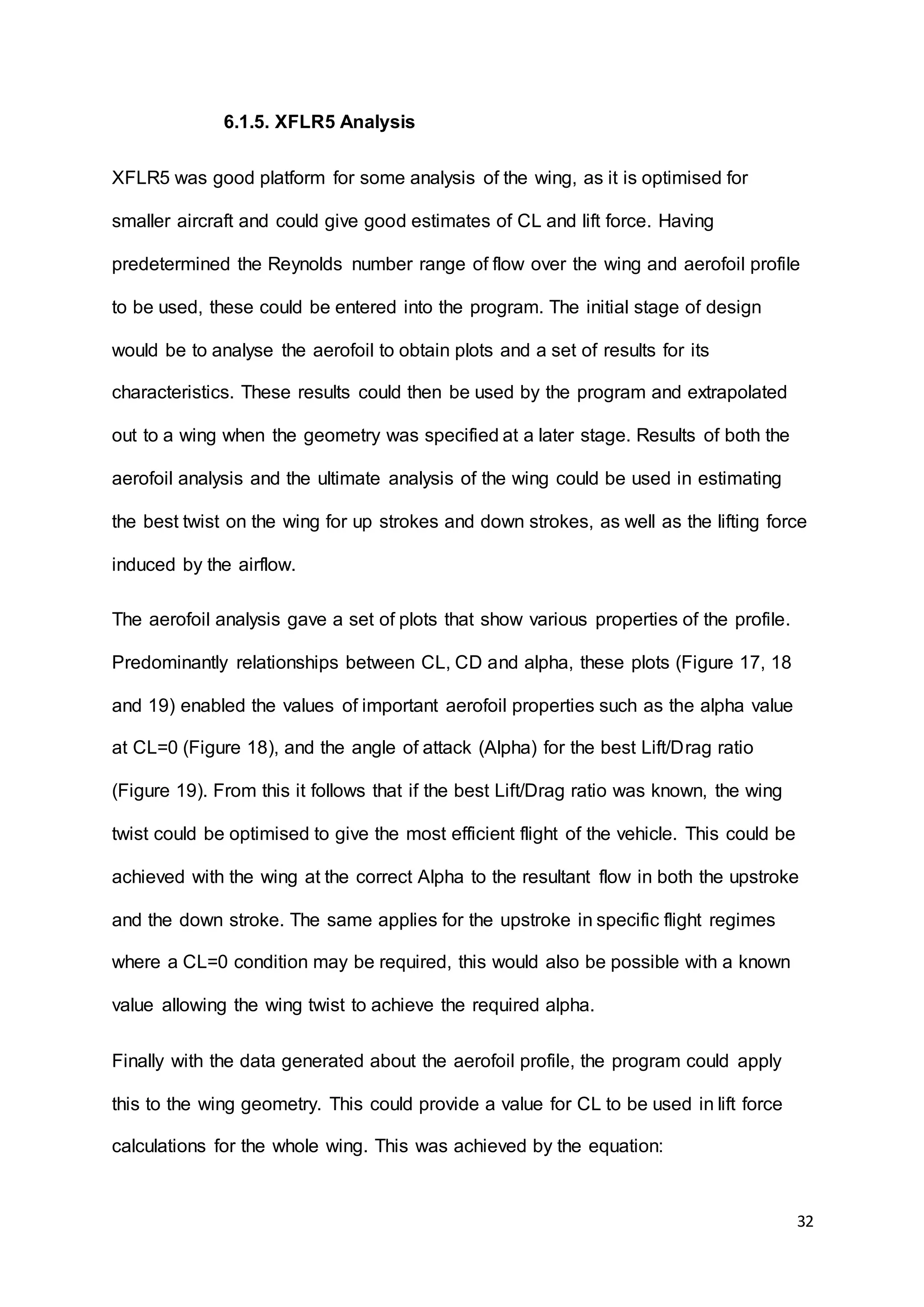
The second study by Dickinson [23] produces approximations for CL and CD in flapping
wing applications (Figure 8). More importantly these are a function of α which due to the
planned servos in the wings, is easy to control. To obtain a theoretical lift force, these
equations can be applied to the predicted or actual α to find an approximation. The CL value
could then be used in conjunction with the lift equation in order to provide a predicted or
theoretical Lift Force.
𝐶𝐿 = 0.225 + 1.58sin(2.13𝛼 − 7.2)
𝐶𝐷 = 1.92 − 1.55cos(2.04𝛼 − 9.82)
𝐿 = 𝐶𝐿
𝜌𝑉2
2
𝐴
Figure 7: Top: J.P.
Whitney projectsthe
theoretical relationship
between φ and α n his
design.Moreof interest
is the phasing of both
sets of motion which
follow a sinusoidal
relationship.This timing
would be good to
replicate in the
experimentalsection of
the project.
Bottom:The plotof
damping forcewith α,
this is the force thatacts
againstthedriving
mechanism. [22]
Figure 8: The approximationsmadeby Dickinson in his workwith the Lift equation
presented below.With a way of measuring Density and velocity aswell as the angle of
attack,theseequationscould beapplied asin workby SaneS.P.[2] to the physicaldata
gathered fromthetest rig and compared to actual values.

19. 19
5.6. Flexibility In Flapping Wings
When comparing wings of aircraft to those found in the natural world, one of the
main differences is the flexibility of bird and insect wings. Insects are typically
characterised with very thin transparent wings with an intricate vein structure to add
rigidity. Whereas bird’s wings consist mostly of feathers with a minority of the wing
surface area being taken up by the bone structure and muscular makeup necessary
for flapping. Feathers typically have a stiff spine to them however this is still not
completely rigid, which allows for a flexible wing. Although studies into natural flyers
initially focussed on defining wings as rigid, studies have now been undertaken to
determine the effects of flexibility.
It has been found that trailing edge flexibility has a considerable effect on the wing
aerodynamics. When a rigid wing translates at a high angle of attack, the leading
and trailing edge vortices periodically generate and shed as found in the results of
(Zhao, et al, 2010) [24]. A wing that has an optimised flexible trailing edge, however
can generate a smaller but much more stable leading edge vortex, with some
parameters out performing rigid wings when used in flapping configurations [24].

20. 20
6. Chapter 1: Methods and Design
6.1. NumericalModelling
Before designing a test rig and wing structure, a numerical analysis of the problem
had to be made. This would provide an indication of the forces acting on the wing. It
was necessary to make calculations, as a critical element to designing a vehicle with
flapping wings would be the lift and thrust achieved, compared to the weight. An
initial estimate for a vehicle weight of 400g was made based on weights of the
notable projects studied in the literature review, most specifically the Festo Smartbird
was considered due to a wealth of information available [3]. With this estimation in
place, the task was to produce a wing and carry out appropriate sizing to produce
adequate lift to support the vehicle in flight. Initial work involved research into
aerofoils, which led into a determination of the Reynolds flow regime the wing would
operate in, this would then be used in XFLR5 to provide results with greater
relevance to a vehicle of the design size. Further theoretical work then required
calculations for resultant flow velocities to find the velocity of induced flow due by
flapping of the wings. This could then be used in XFLR5 to attempt to estimate for lift
force achieved by the test rig at a specific flapping frequency and Angle of Attack
during strokes.
6.1.1. Aerofoil Selection
When selecting a profile for the wing, several considerations had to be made. Firstly
as the project would draw inspiration from biological applications, the profile of the
wing should reflect that of those found in the natural world. Secondly, there would
not be the time or the need for developing a profile unique to the project as a large
variety of aerofoil shapes are readily available for public use. Another consideration

21. 21
would be the strength of material the sections would be constructed from and
tolerances involved with cutting the wing ribs to that profile. These limitations and
criteria required considerable research in order to ensure the right profile was
chosen.
To better understand the characteristics of a bird wing aerofoil, the literature review
aimed to investigate papers where work had been done to obtain a cross section of a
bird wing in flight. The oxford department of zoology [14] achieved this successfully
using a series of cameras around a control volume to obtain an accurate model for
the inner wing of a trained eagle. The result of this study is shown below in Figure 9.
With these findings it was realised that the profile needed to be highly cambered and
have a large leading edge radius and thin trailing edge to correctly replicate the
natural wing. It would also be desirable for the aerofoil to be designed for Low
Reynolds number flow, as based on the vehicles dimensions, it would be expected to
operate somewhere between 𝑅𝐸 1 × 105
and 𝑅𝐸 2 × 105
.
After a search to find a selection of profiles that fitted the already mentioned criteria,
possible candidates were those shown in Figure 10. All aerofoils in this selection are
for Low Reynolds flow, and are highly cambered. The high camber is essential as
the vehicle is operating at low speeds in comparison to conventional aircraft, an
aerofoil with low camber would likely not generate enough lift. As the Reynolds
Figure 9: Aerofoil profiles obtained by
the oxford department of zoology. This
provided a good foundation for the
characteristics to look for in bird-like
aerofoils. [14]

22. 22
number of the flow is low, as well as speed, the amount of drag that a high camber
foil would produce is not nearly as significant as it would be if the same profile was
applied to an air vehicle designed for carrying people.
After reviewing the profiles, two were identified as appropriate for the main wing. The
GOE358 and the Selig 1210 both offered a high camber whilst having enough
thickness to be accurately cut and remain robust in a range of materials. More
importantly this offered the possibility to be laser cut out of wood if desired, which
would be important for rapid production of parts. It was finally decided that the
GOE358 would be more suitable as it has a thicker trailing edge, this would more
conducive to laser cutting if required. The thickness in the aerofoil would be needed
in order to provide enough space for the necessary structure and a servo mounted in
the wing for twisting.

23. 23
6.1.2. Determining Reynolds Number of The Flow Regime
For varying sizes of airborne vehicles, the flow regime that they experience changes.
This is measured by the Reynolds number of the flow. Commercial jets fly in the
regime of 𝑅𝐸 1 × 107
which is considered as high, birds and insects on the other
hand operate at 𝑅𝐸 1 × 103
− 𝑅𝐸 1 × 105
, with insects towards the bottom of the
scale and large birds at the top (Figure 11). Major work in the lower Reynolds
Figure 10: The aerofoil profiles considered for
the design. (1. FX60-100 10%, 2. GM15, 3.
GOE368, 4. GOE63, 5. GOE358, 6. Selig 1210
12%, 7. GOE500) [25]

24. 24
regimes has come about in recent times with the interest in Micro-Air Vehicles, small
unmanned aircraft similar in size to large birds do not experience the same effects as
a large aircraft and must be designed differently.
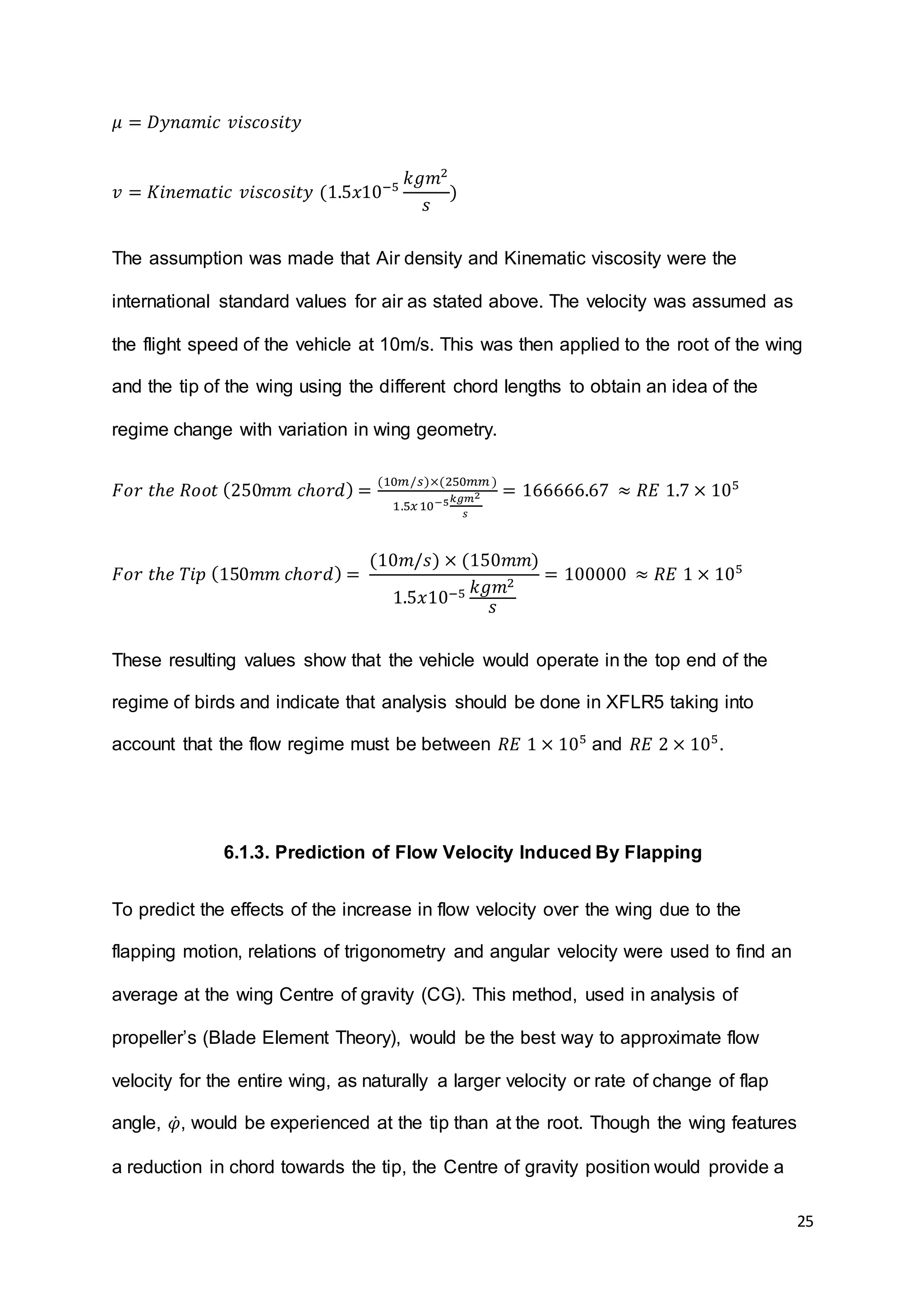
The flow regime can be determined by using the equation stated below which takes
into account the chord of the wing, and velocity of flight.
𝑅𝐸 =
𝜌𝑉𝑙
𝜇
=
𝑉𝑙
𝑣
Where:
𝑅𝐸 = 𝑅𝑒𝑦𝑛𝑜𝑙𝑑𝑠 𝑛𝑢𝑚𝑏𝑒𝑟
𝑉 = 𝑣𝑒𝑙𝑜𝑐𝑖𝑡𝑦
𝑙 = 𝑐ℎ𝑜𝑟𝑑
𝜌 = 𝐴𝑖𝑟 𝐷𝑒𝑛𝑠𝑖𝑡𝑦 (1.225
𝑘𝑔
𝑚3
)
Figure 11: A plot showing theReynoldsnumberagainstthespeed of airborne
body.Thisshowshowvariousapplicationscompare[26].

25. 25
𝜇 = 𝐷𝑦𝑛𝑎𝑚𝑖𝑐 𝑣𝑖𝑠𝑐𝑜𝑠𝑖𝑡𝑦
𝑣 = 𝐾𝑖𝑛𝑒𝑚𝑎𝑡𝑖𝑐 𝑣𝑖𝑠𝑐𝑜𝑠𝑖𝑡𝑦 (1.5𝑥10−5
𝑘𝑔𝑚2
𝑠
)
The assumption was made that Air density and Kinematic viscosity were the
international standard values for air as stated above. The velocity was assumed as
the flight speed of the vehicle at 10m/s. This was then applied to the root of the wing
and the tip of the wing using the different chord lengths to obtain an idea of the
regime change with variation in wing geometry.
𝐹𝑜𝑟 𝑡ℎ𝑒 𝑅𝑜𝑜𝑡 (250𝑚𝑚 𝑐ℎ𝑜𝑟𝑑) =
(10𝑚/𝑠)×(250𝑚𝑚 )
1.5𝑥10−5 𝑘𝑔𝑚2
𝑠
= 166666.67 ≈ 𝑅𝐸 1.7 × 105
𝐹𝑜𝑟 𝑡ℎ𝑒 𝑇𝑖𝑝 (150𝑚𝑚 𝑐ℎ𝑜𝑟𝑑) =
(10𝑚/𝑠) × (150𝑚𝑚)
1.5𝑥10−5 𝑘𝑔𝑚2
𝑠
= 100000 ≈ 𝑅𝐸 1 × 105
These resulting values show that the vehicle would operate in the top end of the
regime of birds and indicate that analysis should be done in XFLR5 taking into
account that the flow regime must be between 𝑅𝐸 1 × 105
and 𝑅𝐸 2 × 105
.
6.1.3. Prediction of Flow Velocity Induced By Flapping
To predict the effects of the increase in flow velocity over the wing due to the
flapping motion, relations of trigonometry and angular velocity were used to find an
average at the wing Centre of gravity (CG). This method, used in analysis of
propeller’s (Blade Element Theory), would be the best way to approximate flow
velocity for the entire wing, as naturally a larger velocity or rate of change of flap
angle, 𝜑̇, would be experienced at the tip than at the root. Though the wing features
a reduction in chord towards the tip, the Centre of gravity position would provide a

26. 26
suitable representation of the entire wing. An explanation of the approach taken is
given below with variables explained in Figure 12.
The initial calculation was to obtain an angular velocity of the gear for a given value
of frequency, 𝑓 (Rotations of the gear that drives the wing per minute). This would be
simply:
𝜔 𝐺 = 𝑓2𝜋
Following on the vertical velocity induced by the linkage between the gear and wing
was found, using the known angular velocity and radius of the gear, 𝑟𝐺 :
𝑉𝐺𝑀𝐴𝑋 = 𝑟𝐺 𝜔 𝐺
From this point, to model the rate of change of flap angle through one period, a good
result could be obtained by using trigonometry to derive the rate of change of vertical
ω 𝑤
𝑥̇
ω 𝐺
𝜑̇
WingSpar
WingHinge
WingCG
Gear
Figure 12: A diagramof the majorcomponentsto detailimportantangularand linear
velocities for finding thevelocity.

27. 27
displacement at the gear linkage, 𝑥̇ (Vertical velocity of the push rod) as the gear
rotates. The top position of the push rod on the gear was taken as 0°
, bottom as 180°
and the left and right as 90°
and 270°
these values map the position of the gear to
the sinusoidal period of flapping experienced by the wing. Positions as shown in
Figure 13.
With a value of velocity induced by the linkage to the wing, the instantaneous
angular velocity of the wing spar could be obtained by:
𝜔 𝑤 =
𝑉𝐺𝑀𝐴𝑋
𝑟ℎ𝑖𝑛𝑔𝑒
Where 𝑟ℎ𝑖𝑛𝑔𝑒 is the distance between the spar connection to the linkage, and the
centre of the hinge.
Applying this angular motion of the wing spar, the vertical velocity of the wing could
be found:
𝜑̇ 𝑀𝐴𝑋 = 𝜔 𝑤 𝑟𝐶𝐺
0°
90°
180°
270°
Figure 13: Angularpositionsshown on thegear.

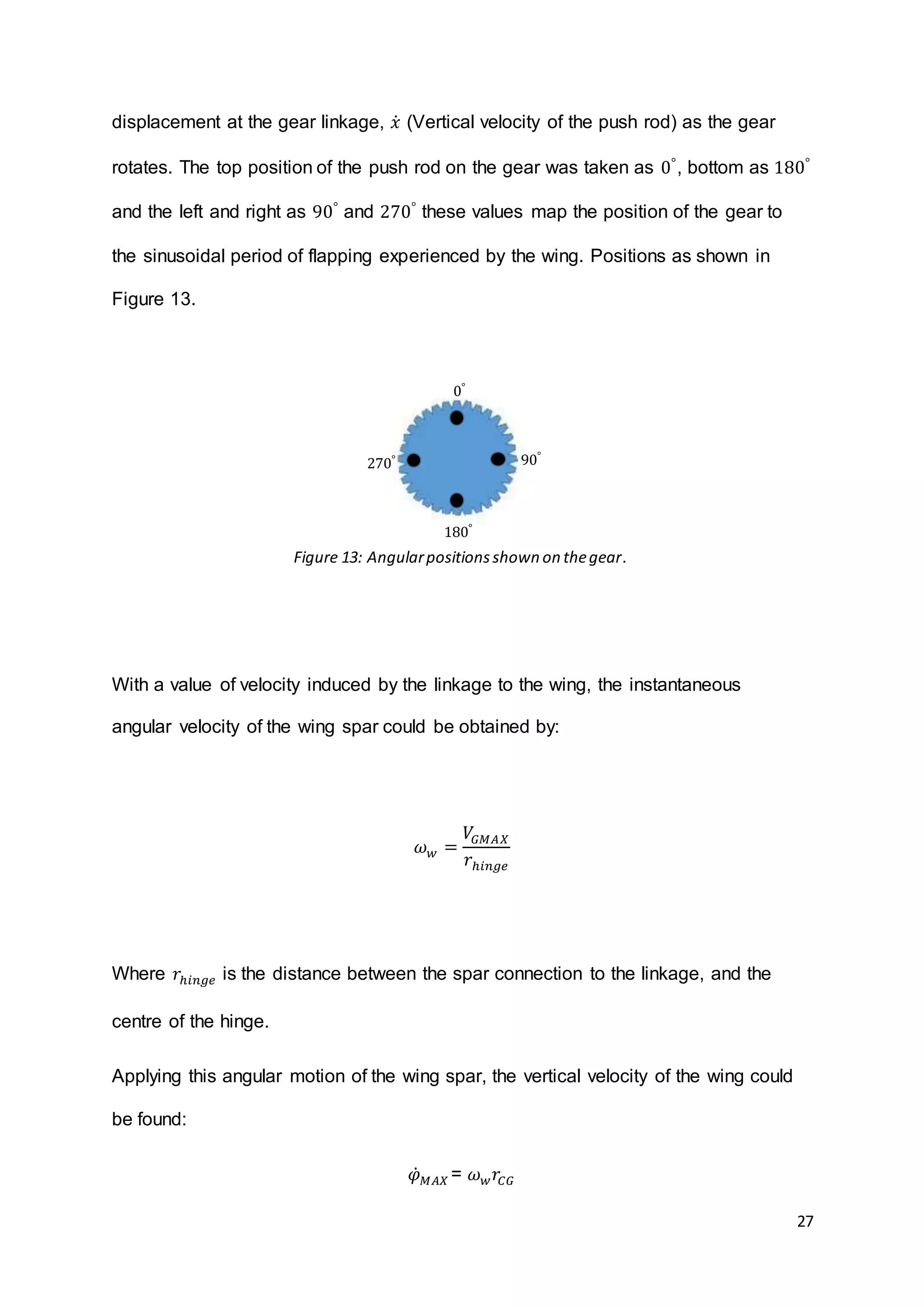
28. 28
Where 𝑟𝐶𝐺 is the distance of the wing span from the hinge to the wing CG.
With the values calculated it is possible to calculate the peak resultant flow velocity
over the wing by using the components of the downward or upward movement of the
wing CG and the free stream flow velocity. These calculations are identical to those
carried out for Blade element theory on aircraft propellers [27], this relies on the
simple trigonometry of an aerofoil moving at a constant velocity, perpendicular to a
freestream velocity generated by the flight speed on the vehicle. This in turn would
produce a resultant effective velocity acting at an angle offset to the freestream.
Although some previous studies have omitted these calculations, many were for
smaller insect like wings. Due to the span of the test rig wings it was felt that the
velocity induced by the wings through their fastest point at the horizontal position
may be significant. This peak velocity could have an effect on the peak lifting force
generated by the wings. This is of interest in this study as the peak force achieved
would give an indication into the feasibility of the concept being adapted to a flying
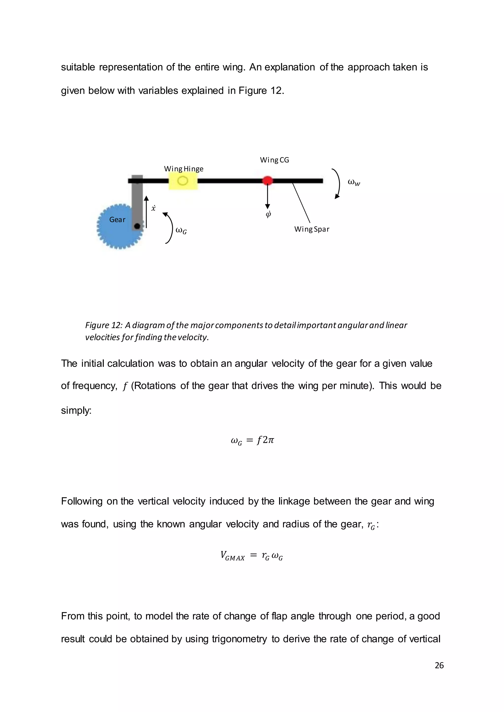
vehicle. In Figure 14 the components of the resultant velocity are shown.
Figure 14: A diagramto showtherelative direction of flow velocities acting
on the wing [28].
𝑉∞
WingCG
𝑉𝐶𝐺 𝑀𝐴𝑋
𝑉𝐶𝐺 𝑀𝐴𝑋
𝑉𝑅𝐸𝑆
Where:
𝑉∞: Free StreamVelocity
𝑉𝐶𝐺 𝑀𝐴𝑋
: Vertical Velocityof WingCG
𝑉𝑅𝐸𝑆: ResultantVelocity
𝛼 𝑅𝐸𝑆: Angle of the Resultantvelocity
fromthe free stream
𝛼 𝑅𝐸𝑆

29. 29
In order to obtain the resultant flow velocity over the wing and its resultant angle, it
was simply a matter of applying Pythagoras, using a given velocity of the freestream,
and trigonometry to find its angle. Below calculations would provide the final inputs
for XFLR5.
𝑉𝑅𝐸𝑆 = √ 𝑉∞
2
+ 𝜑̇ 𝑀𝐴𝑋
2
And
𝛼 𝑅𝐸𝑆 = sin−1
(
𝜑̇
𝑉𝑅𝐸𝑆
)
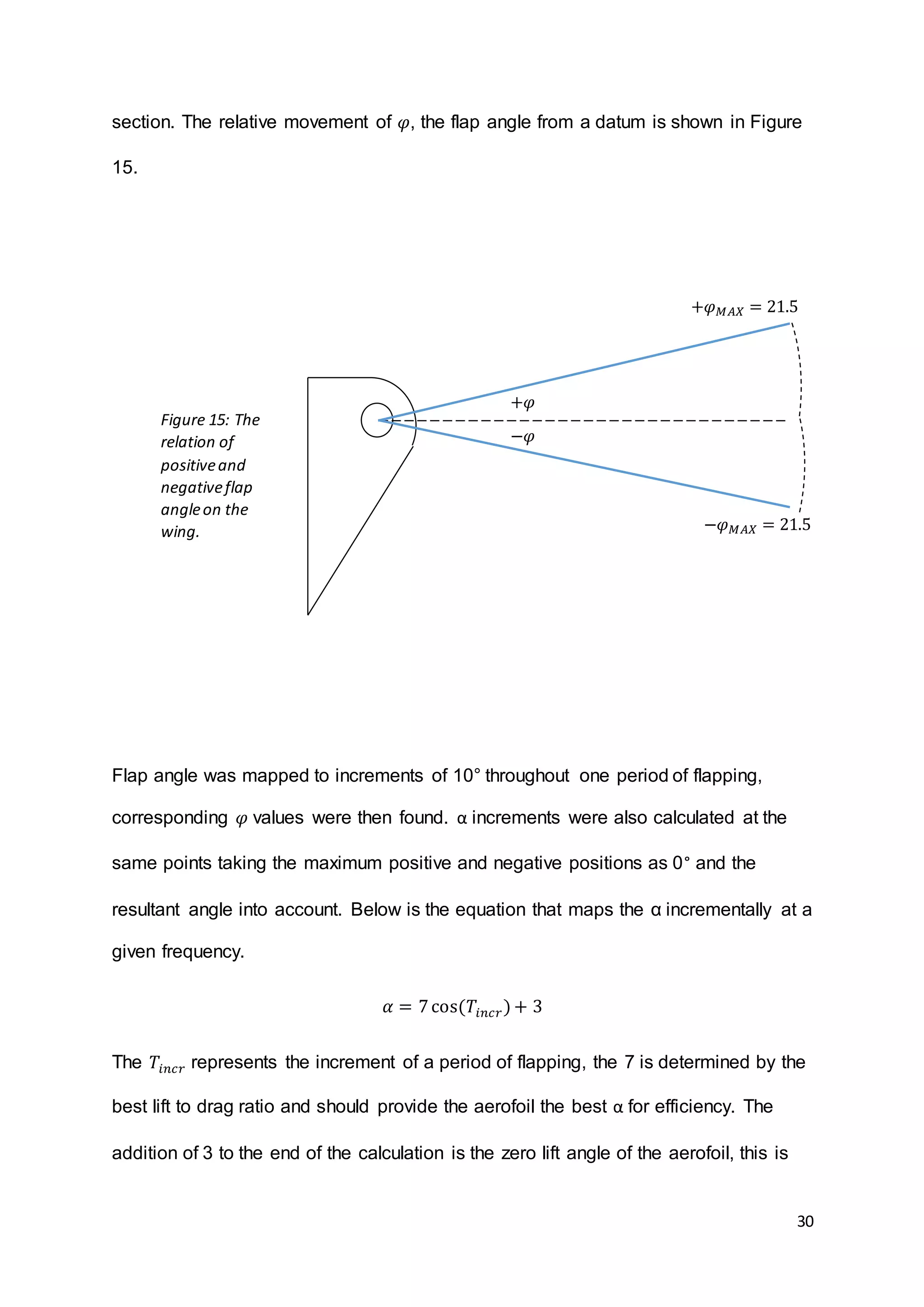
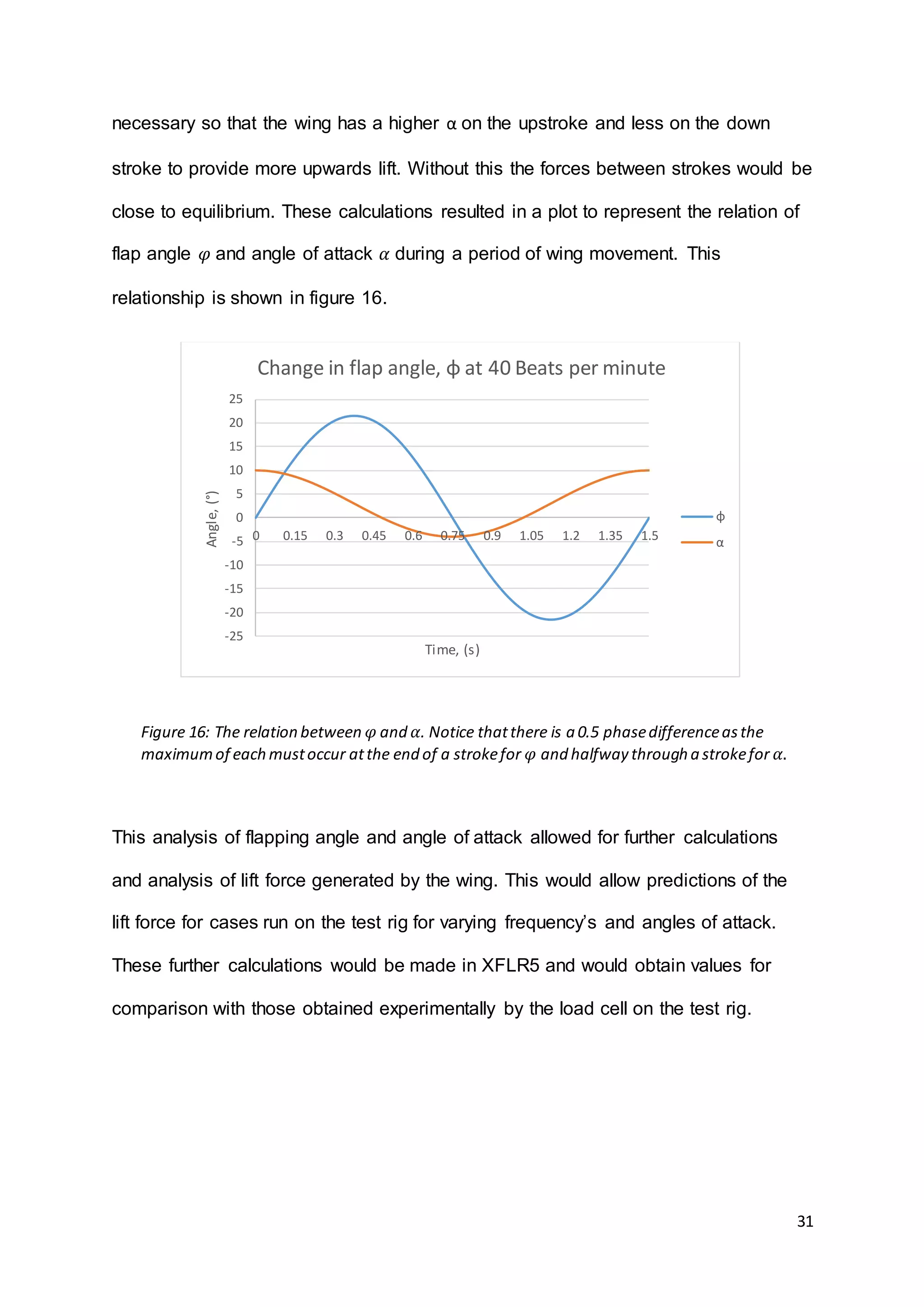
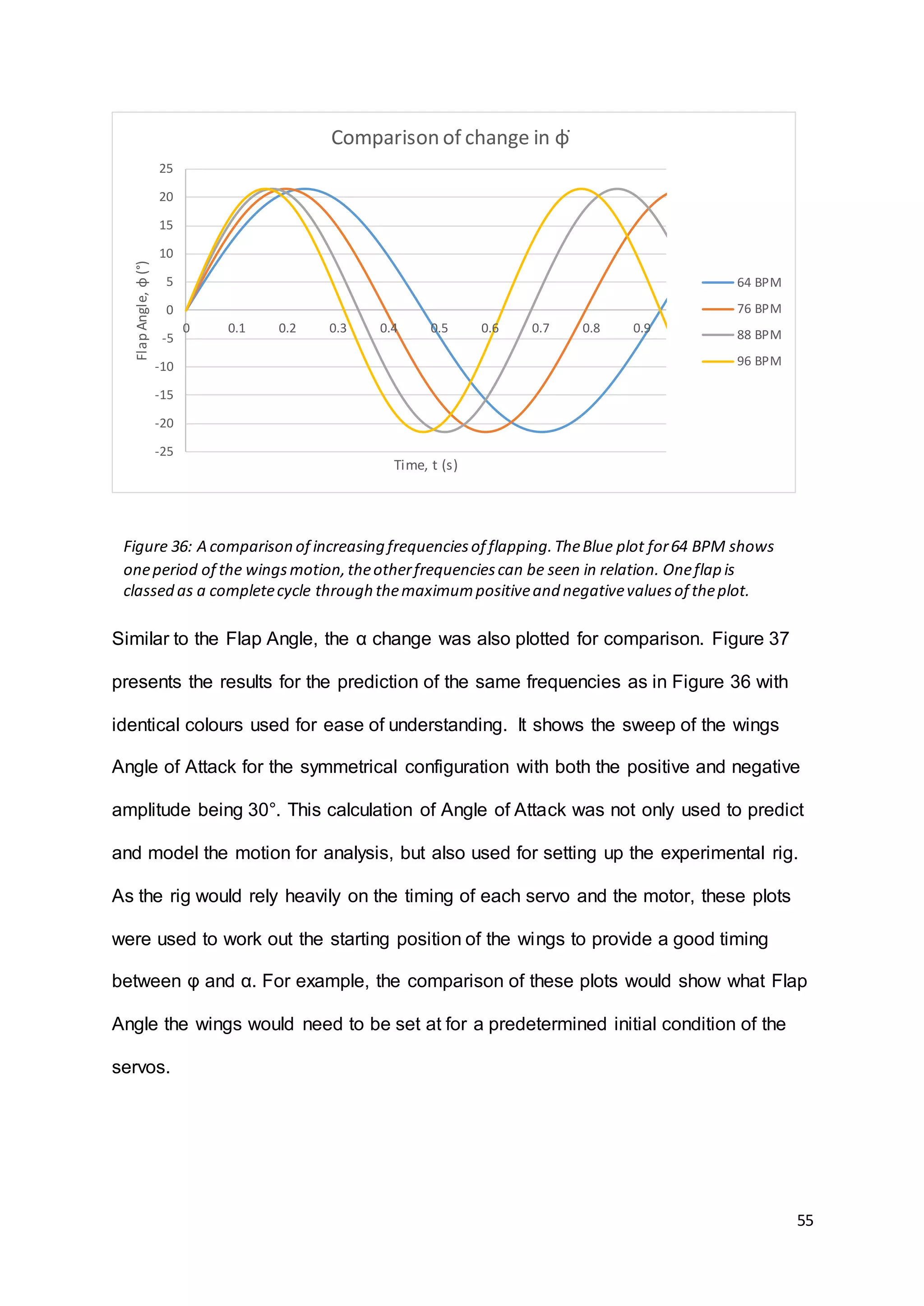
6.1.4. Equations Of Wing Flapping Motion
Having calculated some important elements of flow over the wing, it was also
necessary to determine and plot further characteristics. Using work done by Whitney
and Wood (2011) [22], the relationship between flap angle and alpha through one
period of flapping was calculated for various cases. Particularly the relationship
between flap angle and alpha would be useful as this would need to be recreated in
the control of the flapping motor and the servos for wing twist. The damping force
would also be important as if this was too great, the mechanism and motor would not
be able to withstand and overcome it to drive the wings. Flapping angle when
considered in the context of this study, is the angle of displacement of the wing from
the central datum of its range of movement.
Predominantly used were the equations derived in Whitney and Wood’s conceptual
model for instantaneous lift and damping force. Plots were also created for the
calculated change in flap angle, found by taking the 𝑉𝐶𝐺 𝑀 𝐴𝑋
discussed in the previous

30. 30
section. The relative movement of 𝜑, the flap angle from a datum is shown in Figure
15.
Flap angle was mapped to increments of 10° throughout one period of flapping,
corresponding 𝜑 values were then found. α increments were also calculated at the
same points taking the maximum positive and negative positions as 0° and the
resultant angle into account. Below is the equation that maps the α incrementally at a
given frequency.
𝛼 = 7cos(𝑇𝑖𝑛𝑐𝑟)+ 3
The 𝑇𝑖𝑛𝑐𝑟 represents the increment of a period of flapping, the 7 is determined by the
best lift to drag ratio and should provide the aerofoil the best α for efficiency. The
addition of 3 to the end of the calculation is the zero lift angle of the aerofoil, this is
Figure 15: The
relation of
positiveand
negativeflap
angleon the
wing.
+𝜑
−𝜑
+𝜑 𝑀𝐴𝑋 = 21.5
−𝜑 𝑀𝐴𝑋 = 21.5

31. 31
necessary so that the wing has a higher α on the upstroke and less on the down
stroke to provide more upwards lift. Without this the forces between strokes would be
close to equilibrium. These calculations resulted in a plot to represent the relation of
flap angle 𝜑 and angle of attack 𝛼 during a period of wing movement. This
relationship is shown in figure 16.
This analysis of flapping angle and angle of attack allowed for further calculations
and analysis of lift force generated by the wing. This would allow predictions of the
lift force for cases run on the test rig for varying frequency’s and angles of attack.
These further calculations would be made in XFLR5 and would obtain values for
comparison with those obtained experimentally by the load cell on the test rig.
-25
-20
-15
-10
-5
0
5
10
15
20
25
0 0.15 0.3 0.45 0.6 0.75 0.9 1.05 1.2 1.35 1.5
Angle,(°)
Time, (s)
Change in flap angle, φ at 40 Beats per minute
φ
α
Figure 16: The relation between 𝜑 and 𝛼. Notice thatthere is a 0.5 phasedifferenceasthe
maximumof each mustoccur atthe end of a strokefor 𝜑 and halfway through a strokefor 𝛼.

32. 32
6.1.5. XFLR5 Analysis
XFLR5 was good platform for some analysis of the wing, as it is optimised for
smaller aircraft and could give good estimates of CL and lift force. Having
predetermined the Reynolds number range of flow over the wing and aerofoil profile
to be used, these could be entered into the program. The initial stage of design
would be to analyse the aerofoil to obtain plots and a set of results for its
characteristics. These results could then be used by the program and extrapolated
out to a wing when the geometry was specified at a later stage. Results of both the
aerofoil analysis and the ultimate analysis of the wing could be used in estimating
the best twist on the wing for up strokes and down strokes, as well as the lifting force
induced by the airflow.
The aerofoil analysis gave a set of plots that show various properties of the profile.
Predominantly relationships between CL, CD and alpha, these plots (Figure 17, 18
and 19) enabled the values of important aerofoil properties such as the alpha value
at CL=0 (Figure 18), and the angle of attack (Alpha) for the best Lift/Drag ratio
(Figure 19). From this it follows that if the best Lift/Drag ratio was known, the wing
twist could be optimised to give the most efficient flight of the vehicle. This could be
achieved with the wing at the correct Alpha to the resultant flow in both the upstroke
and the down stroke. The same applies for the upstroke in specific flight regimes
where a CL=0 condition may be required, this would also be possible with a known
value allowing the wing twist to achieve the required alpha.
Finally with the data generated about the aerofoil profile, the program could apply
this to the wing geometry. This could provide a value for CL to be used in lift force
calculations for the whole wing. This was achieved by the equation:

33. 33
𝐿 = 𝐶 𝐿
𝜌∞ 𝑉2
2
𝐴 𝑊
As XFLR5 provides the option for specifying the density, freestream velocity and the
wing area being determined by the design. All values in this equation were known
leading to just a single run for each case in the program being needed to find the lift.
This was useful when compared to the predicted weight of the vehicle to find out if lift
generated by the wings would be sufficient. The 3-Dimensional plots generated
would also aid in structural design as they would detail the panel forces across the
mesh, this would reveal the areas of the highest force (Figure 20). Other plots that
were of interest were also available such as those of coefficient of pressure, surface
velocity and streamlines of flow in the wings wake. However these were not essential
to the project as they would be inaccurate for the instantaneous cases that were run
for various data points.
Figure 17: The CL vs CD plot for the
aerofoil profile used on the wing.

34. 34
Figure 18: CL vsAlpha,this is usefulto
determinethe maximumeffectiveangleof
attackof the wing beforeit beginsto stall.
Figure 19: Perhapsthemostusefulplotgenerated,theCL/CD vs α, this showsthe
mostefficient angleof attackof thewing beforetherelationship between lift and
drag deteriorates.

35. 35
Before Analysis could be made on the wing model, a mesh analysis had to be
carried out comparing CL to the amount of panels used to build the wing model.
There would be a relationship between results for CL and the amount of panels
used, with results eventually converging to a value as the number of panels was
made greater. This point had to be determined as it would indicate the optimum
Figure 20: A plot of the
panelforces acrossthe
wing at the top of the
upstroke.Noticethe
information given
including dataabout
the geometry of the
wing,results of the
analysisand a key for
interpretation of the 3D
plot.
Figure 21: A plotfor CP (Coefficientof pressure) Figure 22: Surface velocityplot
Figure 23: The streamlineplot for
the wing,showing thewingtip
vortices.

36. 36
mesh configuration for providing accurate results with the least computing power
needed. The final mesh and the results of the mesh analysis are shown in Figure 24.
6.2. Design
The basic concept for the design of the test rig was taken from findings in the
literature review, and how best to achieve the fundamental aims of the project. Most
examples of previous work use a simple straight set of wings directly connected to
the internal mechanism. This configuration was decided on for the design of the test
rig, not only as a result of these findings, but also for obtaining a symmetrical lifting
force and for simplicity of design. An articulated wing has many more moving parts
0.49
0.5
0.51
0.52
0.53
0.54
0.55
0.56
0 500 1000 1500 2000
CL
Number of Panels
Mesh Analysis
Figure 24:
Left: The XFLR5 modelof the wingswith
the finalmesh.
Below: The resultsof themesh analysisof
numberof Panelsvs CL.Note theplot
convergesto a valueof 0.556. This
determinesthe numberof panelsas1820.

37. 37
which would need to be fitted correctly, as well as the distances of the pushrods in
the wing refined to a very high precision.
6.2.1. CAD Modelling
The overall configuration of the testing rig would consist of a mechanism driven by a
motor to flap the wings, with servo motors to twist the wings accordingly. This would
simplify the control of the wings, but still enable control of the frequency and the twist
for angle of attack. With this in mind, work on the design for the test rig began first
and foremost with research into components that could not accurately be made in
house. Largely, this meant the gears for transmission of the rotary motion of the
motor, to the wings. Once the size of gears was known, other components could be
sized appropriately.
With the aerofoil profile and wing geometry being decided by previous work, design
of the structure took place within Solidworks. This approach had a number of
benefits, including the ability to visualise and check the design before fabrication, as
well as providing accurate part files for precise machining of components. A further
benefit of the software, was the capability to animate the model and simulate motor
motion on parts. This allowed motion to be checked and refined thoroughly as well
as close inspection for any interference between moving parts. The final assembly
model is shown in Figure 25.

38. 38
When designing the individual parts for the structure, some parts would be used as
they were purchased, needing either a very basic level of machining or none at all.
An example of this was the carbon rods used as spars in the wings, these were
simply purchased and cut to size. To avoid issues with fitting these parts with others,
they were reproduced in the CAD software so they could be placed in an assembly
file with all the other components. This allowed the tolerancing of the parts as cutting
would not be completely accurate, such as the wing ribs, where holes for the spars
would be made 0.2mm larger than the carbon rod to ensure a proper fit (Figure 26).
This approach needed to be taken for almost all areas where parts would fit together,
as even though the 3D printing and laser cutting machines used are very precise,
they still have a limited accuracy meaning parts may come out slightly larger or
smaller than designed.
Figure 25: The CAD model of the final assembly of the test rig. This model was animated and had the possibility of
moving constrained parts by dragging them. This proved extremely valuableto the design process.

39. 39
The use of the CAD model was invaluable to machining the wooden parts of the
design and 3D printing the hinges. These components have complex geometries
which may have been hard to achieve using traditional machining and cutting
techniques (Figure 27). The Ribs have an aerofoil shape that is highly cambered with
a thin trailing edge, this would be almost impossible to do accurately by hand. As
well requiring precision for their basic shape, the ribs and frames also involved some
intricate cut outs which were only made possible by the laser cutting machine. The
shape of the ribs and frames are shown in Figure 28.
Figure 26: The tolerancein
the CADmodel on the front
sparof the wing is shown
with a very obviousgap
between the sparand edges
of the hole. This accounts
forerror in thespar
diameterand the cutting of
the wooden parts.
Figure 27: The separate
assembly of thewing made
the finalassembly of the
wholetest rig much easier
to produce.Thisalso shows
the complexityof the rib
shapes.

40. 40
6.2.2. Materials
The selection of materials is an essential phase to any design and is subject to many
considerations. Parameters such as cost, machinability, structural strength,
availability and density were all considered in the selection of materials for the wings
and frames. Considerations were made for each part as to what the loads and
stresses might be, which allowed the qualities of the material to be prioritised. This
can be seen in the final design and prototype by the use of carbon, plywood and
balsawood for different elements in the structure.
The ribs of the wing are primarily responsible for maintaining the profile of the wing.
This requires them to be good at holding their shape under load. The loads
experienced by the ribs however, are relatively much lower than those found in the
spars, therefore it was decided that the ribs could be constructed from lightweight
birch plywood. This has good strength for the requirements of the wing ribs and
could easily and accurately be laser-cut to size straight from the CAD model in
house (Figure 28). As the model was to be a one off prototype, purely for testing, it
Figure 28: The
laser cut parts
forthe Ribs and
Frameswith the
highly cambered
aerofoilprofile
and complex cut
outs.

41. 41
would not be necessary to use Carbon fibre due to the much higher cost of buying
and cutting the material, as well as the difficulty in machining the parts.
The frames were constructed from the same birch plywood. Laser cutting was also
the easiest method for cutting these components due to the accuracy required for
distances between holes as well as the irregularly sized cut-outs.
For the spars, carbon tubes were selected as these offered good strength against
the loads experienced by a flapping wing. Although the flapping wing would be
considerably smaller and therefore subject to much smaller loads than conventional
full size aircraft, the wings motion might induce loads that were beyond the
capabilities of plywood. The carbon rods due to their cylindrical geometry, would also
provide good stiffness which would be important for the wing to maintain its shape
and strength throughout a flap cycle.
Balsawood was also used in the design, however no major structural components
were made from balsa. The use of this material is simply to support the wing
covering at the leading and trailing edge and enable the covering to be attached
securely.
6.2.3. Weight Estimation
A calculation of the weight was essential for several aspects of the project. As the
majority of parts had been designed in Solidworks, it was easy to use the data
available from the programme in order to determine the physical properties of the
individual parts. This would allow for an accurate estimation of the overall weight of
the entire structure. The volume of the parts would be used with the known average
density of its material, in Solidworks it was also possible to obtain data on the

42. 42
centroid of a part or structure which would be useful when calculating moments of
the centre of mass.
First and foremost the weight estimation would be used when determining the
capacity of load cell required for testing. This was necessary to ensure that the setup
was optimised to achieve the best results. Using a load cell with a capacity too large
would lead to inaccurate measurements, whereas using a capacity that is too small
could damage the measuring equipment or lead to obtaining an incomplete set of
results.
A second purpose of the weight estimation would be in the calculation for its
feasibility. If the lift results found in testing were to show that enough force was
produced to lift the weight of the test rig, it is feasible that it could be converted into a
flight vehicle. Optimisation could then take place to investigate for any improvements
to be made. If the test rig was found to be too heavy, a successful flight vehicle
would require the material and geometry of the parts to be changed, or the structure
redesigned.
The estimation of the individual component weights is included below in Figure 29.
The estimated assembly weights are in Figure 30 with comparison to the actual
weight. Note that the wings came out lighter than predicted, this was due to the
difficulty in predicting the exact density of the wood and the loss of material from the
cut outs in the ribs. The frame however came out heavier than expected, this is
partially due to the extra wooden spacers needed to give the frame rigidity, and
minor design changes that were made to the assembly to give the gears a more
functional arrangement.

43. 43
Component Weight Estimation
Wing
Rib 1 14.1 g
Rib 2 9.7 g
Rib 3 11.6 g
Rib 4 7.9 g
Rib 5 6.6 g
Rib 6 5 g
Front Spar 7.1 g
Centre Spar 37.6 g
Servo 53 g
Frame
Frame 1 31.7 g
Frame 2 31.7 g
Motor 53 g
Carbon rods 10.7 g
Gears 25 g
Assembly Estimation Actual
Left Wing 76.3 65 g
Right Wing 76.3 65 g
Frame 152.1 177 g
Figure 29: Table of component weight estimation
Figure 30: Table of Assembly weightestimations

44. 44
6.2.4. Control
In order to conduct the testing accurately and precisely, a good degree of control
was needed over the test rig. Previously mentioned was the motor and two servos
included in the design which were to control wing flapping frequency, and the angle
of attack of the aerofoil respectively. In order to obtain good results that could be
compared to the theoretical cases predicted in the numerical modelling, the
frequency needed to be kept as a constant and the angle of attack consistently
changing between pre-set values.
The solution to control was the use of an Arduino board which could be programmed
to run the tests autonomously. The Digital outputs were capable of operating the
motor and servos by the use of the ‘write()’ command. This command was important
as once an object had been specified as a servo, and the servo library imported, it
would simply use a value representing degrees of servo movement to operate the
wings. Therefore, for the servo motors, this was as simple as specifying the
movement in degrees, with ‘write(90)’ being the zero angle of attack position of the
wings. The ESC (Electronic Speed Controller) and Motor also had function similar to
the Servos, with a simple calibration allowing the number of degrees specified to
equate to a percentage of the motor speed. This was achieved via the digital outputs
on the board which would generate the signal to be interpreted by the components.
The programmable nature of the board allowed for a function to be written for the
sweeping of the servos back and forth. This meant that they would not have to be
manually controlled and greatly aided the repeatability of each case as the speed of
the sweep and its magnitude could easily be set.

45. 45
An example of a test case to be programmed into the board is shown below in
Appendix 3.
The code shown in Appendix 3 has 3 main lines of code that control the motor and
the servo motors. These 3 lines are the most important with regard to test cases
being run with the flapping and wing twisting in synchronisation, as they control
motor and servo speed, along with the minimum and maximum values of the servos.
The line controlling motor speed is shown below:
escmot.write(43);
In this line, the motor has been related to the servo library with the name ‘escmot’
and associated to a digital output pin of the Arduino. The write command then
specifies the angle that would be signalled to the motor which acts as a servo, in this
case 43. From testing it was found that different angles written to the motor would
give varying motor speeds and these were appropriately calibrated to give a list of
‘write()’ values for corresponding frequency in wingbeats per minute, for the example
above, 43 gives a frequency of 60 beats per minute.
The other lines of importance were as follows:
for(pos = 70; pos < 170; pos +=3.5)
for(pos = 170; pos >= 70; pos -=3.2)
These parts of the code determine the change of the variable ‘pos’, this variable
changes depending on the current position of the servo, and adds or subtracts the
end value depending on the instantaneous state of the servo. This variable is then
used to input back into the servo and creates and autonomous sweep back and forth
of the servo arms. In the case of the examples given, the addition and subtraction
values for degrees of the servo is 3.5 and 3.2 respectively. This essentially specifies

46. 46
how many degrees the servo arm moves every loop of the code. A 15 millisecond
delay is included to allow the servo time to act accordingly. The 70 and 170 define
the limits in degrees the servo may sweep, in this case the wing can achieve up to
30° negative angle of attack and 70° positive, this occurs as for the servos mounted
in the wings, a 0° angle of attack is achieved at pos=100. It follows that the first line
specifies an increase in increments of 3.5° from a servo position of 70° to 169°, and
the second line a decrease of 3.2° for the wing servo moving back from 170° to 70°.
The difference in what is effectively the speed of the servos movement, is a result of
the wing travelling faster in one direction than the other as it has gravity to aid it in
the down stroke.
6.2.5. Electronics
Once a program had been written to control the test rig, the final stage was to wire
up the motors and breadboard accordingly. This was important as improper wiring
could cause the servos to move in the wrong direction, or could potentially damage
the Arduino should the power supply to the ESC be connected wrong. As it was
found that the 5 volt power supply of the Arduino board was enough to power the
servos, this only left the ESC and motor needing to be powered by an alternative
source.
It was important that the brushless motor received a consistent power supply from
the power source via the ESC. The power supply from the Arduino although
sufficient to power the servo motors, could not power all three motors, therefore an
alternative source was needed. Initially a 9V battery was used, which proved
adequate to power the motor, however it was quickly drained and did not provide a
consistent current and voltage. For this reason a power supply was used with a

47. 47
variable current and voltage, this was the perfect solution providing a uniform voltage
and current as well as enabling changes to be made with ease. It was important that
this power source did not come into contact with the Arduino board as it could easily
damage it, either with excessive voltage or current. For this reason the power supply
was connected straight to the ESC rather than going through the breadboard which
took away the risk from an error in the connections.
Another issue in terms of electronics was the load cell used for measurement of
results. This required a nominal voltage of 10 volts to function and was therefore
connected to a separate power supply that would feed a consistently. This would
keep results as accurate as possible as it avoided any potential variation in the
voltage which could be picked up by the oscilloscope measuring the output. The load
cell also had two wires for output voltage, it was these wires that were connected to
the oscilloscope to obtain a readable signal. With one wire being for positive and the
other wire for negative, this allowed the load cell to measure both compressive and
tensile forces. These output wires had a capacitor between them, this was necessary
as the signal was initially found to be quite ‘noisy’. The capacitor served the purpose
of smoothing out the signal, reducing the amplitude of oscillations and making the
detectable frequency limit considerably lower.
Figure 31 shows a diagram of the circuit for the test rig. The associated power
supply connections for the ESC and brushless motor are also shown. All the
connections were kept as simple as possible and arranged neatly to avoid mistakes
when connecting the circuit to set up the test rig. Also of importance was the correct
motor being connected to the correct digital output pin, this was important as if the
motor was to receive a signal for one of the servo motors it would have potentially

48. 48
caused damage to the test rig by too many revolutions per minute inducing
excessive frequency to the wings.
6.2.6. Measurement Of Results
It was decided early in the beginning of the project that measurement would be
undertaken by use of a load cell. A load cell could be used in the place of strain
gauges mounted on a support of the test rig, this would have the effect of removing
the complications of properly installing strain gauges as well as providing a more
accurate measurement of vertical forces exerted by the flapping wings. This would
come as a result of the load cells specific measurement of force exerted in a single
direction rather than the strain in a material as a result of that force.
Figure 31: The diagramof thecircuit required for the controlof the test rig with the codein
Appendix 3.(Yellow and orangewiresrepresentsignal wires,red is positive,blackor brown are
ground wires)

49. 49
The load cell required some initial set up. In order to amplify the voltage from the
output, a circuit was constructed that increased the strength of the signal by a
thousand times through a series of resistors, a H-bridge and an alternative power
supply. This took the signal received on the oscilloscope from the order of millivolts
to volts which, in conjunction with a capacitor, greatly reduced noise in the signal and
provided a more accurate reading. With this circuit providing a good signal from the
load cell, it was then calibrated using known masses and measuring the output
voltage (Figure 32). As the limit of the load cell was 20N (2kg) increments of weight
were added up to a maximum of 17N (1.7kg.), to avoid reaching the load cell limit.
This calibration was to confirm that the equipment specification was correct and the
relationship between output voltage and force exerted was linear.
0
0.5
1
1.5
2
2.5
3
3.5
4
0 2 4 6 8 10 12 14 16 18
Volts(V)
Force (N)
Volts/Newtons
Volts/Newtons
Figure 32: The Load cell calibration showing therelationship between voltagesreceived fromthe
outputof thedevice and the forcesapplied.

50. 50
7. Chapter 2: Results
7.1. Results Of Numerical Analysis
7.1.1. Theoretical Relationship of Flap Angle and α
To optimise the Lift Force achieved by the test rig, it was essential that there was a
good synchronisation between change in Flap Angle and change in Angle of Attack.
To do this, a correct configuration for the Angle of Attack was calculated for various
points throughout one period and an appropriate sinusoidal function was generated
to model the sweeping motion replicated by the servo. By thinking about the flow
over the wing and the Angle of Attack induced by the wings vertical reciprocating
motion, it follows that the best configuration for the upstroke would be a steep
positive Angle of Attack to minimise negative air resistance forces. The down stroke
would require a negative Angle of Attack due to the vertical component of velocity
and the resulting angle of effective flow. Both the top and bottom of the strokes
would require an Angle of Attack of 0°. For this reason, the sinusoidal functions of
both the Flap Angle φ, and Angle of Attack α, would need to be exactly one half of a
period out of phase. This is shown in the following figures of results from the
numerical analysis.
Due to the challenge of obtaining results for a wide range of configurations
experimentally, the number of cases run would be limited. The solution was two
studies, one for the effect of increasing Angle of Attack, the other which would be for
rate of change of Flap Angle (frequency). The frequency study would be repeated
over four different frequencies with two different servo programmes. One of these
would be a symmetrical sweep of Angle of Attack between +30° and -30° (In
programming the servo, 0° for the wing was at 90° rotation for the servo making this

51. 51
case 60° - 120°). The other would be a larger sweep with a steep Angle of Attack
during the upstroke between +70° and -30° (For the same reason as before, the
angle felt by the servo this would be 60° – 160°). In real terms, the first case would
be more similar to a bird in a cruising phase of sustained flight, the second would be
more similar to take off, with more lift required and less resistance on the upstroke.
These tests would be run in a static condition with an effective freestream velocity of
0 m/s suggesting that the second pattern of movement might yield better lift results,
being more similar to technique used by birds in a similar condition.
Below (Figure 33) is an example of the relationship between φ and α when the wings
are at a frequency of 64 Beats per minute. It can clearly be seen from the plot of the
results that the function for α is exactly half a period out of phase with φ. The
symmetrical sweep on the servos applied in this model means the positive and
negative amplitude of α are the same. This configuration as mentioned before is
more similar to a bird in a sustained period of flight, with a constant airflow forming a
horizontal component over the chord of the wings. For this case, the sinusoidal
relation to Flap Angle for the Angle of Attack is as follows:
𝛼 = 30cos( 𝜑)

52. 52
Figure 34 shows a different configuration of Angle of Attack during one cycle of
flapping (A full wing beat through the upstroke and downstroke). The input angles to
the servo in this case were 60-160, creating a sweep of the wing through from +70°
to -90° α. This greater amplitude in Angle of Attack is more similar to that seen in bird
wings during take-off and climb at low velocity. When reproduced experimentally a
better Lift Force was expected, as the test rig would operate in stationary flow
conditions. Notice in Figure 34 that the phasing of both parameters is identical to that
of Figure 33, but here the function of α has been altered to give a larger positive
amplitude. The function was altered as below:
𝛼 = 50 cos( 𝜑) + 20
-40
-30
-20
-10
0
10
20
30
40
0 0.15 0.3 0.45 0.6 0.75 0.9
Angle,(°)
Time, (s)
Change in φ and α (64BPM-Sweep:60-120)
φ
α
Figure 33: Plotof
Flap Angleand
angleof attack
forthe test rig at
64 beatsper
minutewith a
symmetrical
servo sweep for
angleof attack.

53. 53
Calculations were also made to provide a representation for φ with an increasing
value of α. For this study into increasing Angle of Attack, the sweep of α was kept
symmetrical from the centre of the servo range. These cases would be kept to the
same frequency to allow the measurement of change with a single parameter, this
meant the motor speed was to be kept constant through all the tests at 88BPM. The
measurements taken would confirm the amount of twist to be applied to the wing for
the best lift production with the induced airflow over the wing. Figure 35 shows the
theoretical relationship of the two parameters for the study into Angle of Attack
variation.
-40
-30
-20
-10
0
10
20
30
40
50
60
70
80
0 0.15 0.3 0.45 0.6
Angle,(°)
Time, (s)
Change in φ and α (96 BPM-Sweep:60-160)
φ
α
-60
-40
-20
0
20
40
60
0 0.2 0.4 0.6
Angle,°
Time, s
Flap Angle and Increasing α sweep against
Time
Flap angle
α=10
α=20
α=30
α=40
α=50
Figure 34: Plotof
Flap Angleand angle
of attackfor thetest
rig at 96 beatsper
minutewith an
asymmetricalservo
sweep creating a
greaterα on the
upstroke.
Figure 35: Flap Angle
againsttheincreasing
stepsof α. Notethatthe
plotsof alpha showa
symmetrical.

54. 54
The other parameter that would be investigated would be the rate of change of Flap
Angle𝜑̇. This is directly linked to the frequency of the flapping which is mostly
referred to as Beats per Minute (BPM) of the wings in this paper. The theory behind
𝜑̇is that when the wings beat faster, the cumulative force they exert over the space
of a minute would be greater due to a higher number of cycles. This is similar to a
higher number of revolutions in an engine. However, with a higher frequency the
wings also move faster through the air vertically, which would have the effect of
slightly increasing the force generated by each flap. Figure 36 shows the modelling
of higher frequency flapping, it can be seen from the plots for the increasing BPM,
that 96BPM will lead to almost a whole extra period in the sinusoidal motion of the
wing over 64 BPM. It follows that in theory the wings could generate twice the force
at 96 BPM, with an increased airflow velocity and the wings beating double the
amount of times within the same time period. The frequencies plotted here were
determined by the inputs to the motor from the Arduino. This was done as if entering
angles to a servo, and to avoid over stressing the mechanism of the test rig, the
inputs were kept below a certain value as its loss would have been fatal to the limited
timescale for the project.

55. 55
Similar to the Flap Angle, the α change was also plotted for comparison. Figure 37
presents the results for the prediction of the same frequencies as in Figure 36 with
identical colours used for ease of understanding. It shows the sweep of the wings
Angle of Attack for the symmetrical configuration with both the positive and negative
amplitude being 30°. This calculation of Angle of Attack was not only used to predict
and model the motion for analysis, but also used for setting up the experimental rig.
As the rig would rely heavily on the timing of each servo and the motor, these plots
were used to work out the starting position of the wings to provide a good timing
between φ and α. For example, the comparison of these plots would show what Flap
Angle the wings would need to be set at for a predetermined initial condition of the
servos.
-25
-20
-15
-10
-5
0
5
10
15
20
25
0 0.1 0.2 0.3 0.4 0.5 0.6 0.7 0.8 0.9
FlapAngle,φ(°)
Time, t (s)
Comparison of change in φ ̇
64 BPM
76 BPM
88 BPM
96 BPM
Figure 36: A comparison of increasing frequenciesof flapping.TheBlue plot for64 BPM shows
oneperiod of the wingsmotion,theotherfrequenciescan be seen in relation. Oneflap is
classed as a completecycle through themaximumpositiveand negativevaluesof theplot.

56. 56
The last representation to be generated was the combined plot for φ and α (Figure
38). This enabled the above two figures (Figures 36 and 37) to be seen as one.
Although somewhat busy, it does show how quickly the change in α could become
out of phase with φ, as viewing a mismatching frequency for Flap Angle and α
reveals. This plot shows the amplitude of the large range of servo sweep from 60° to
160°, where the amplitude on the upstroke was to give the wing a very high positive
Angle of Attack at 70°. The twist of the wing to achieve this condition had to happen
at a considerably increased rate, in order to do this the lines of code referred to in
the methods chapter, had to be altered to allow a faster sweep of the servo arm.
Typically this involved increasing the degree increments from in the region of 3.0 to
around 4.5-5.0. This meant the servo arm would move further every time the code
loop was executed and therefore the sweep was faster.
-40
-30
-20
-10
0
10
20
30
40
0 0.1 0.2 0.3 0.4 0.5 0.6 0.7 0.8 0.9
α,(°)
Time, (s)
Comparison of change in α for Servo Sweep: 60°-120°
64 BPM
76 BPM
88 BPM
96 BPM
Figure 37: The comparison of frequenciesfor changein α, or the sweep of the servo.

57. 57
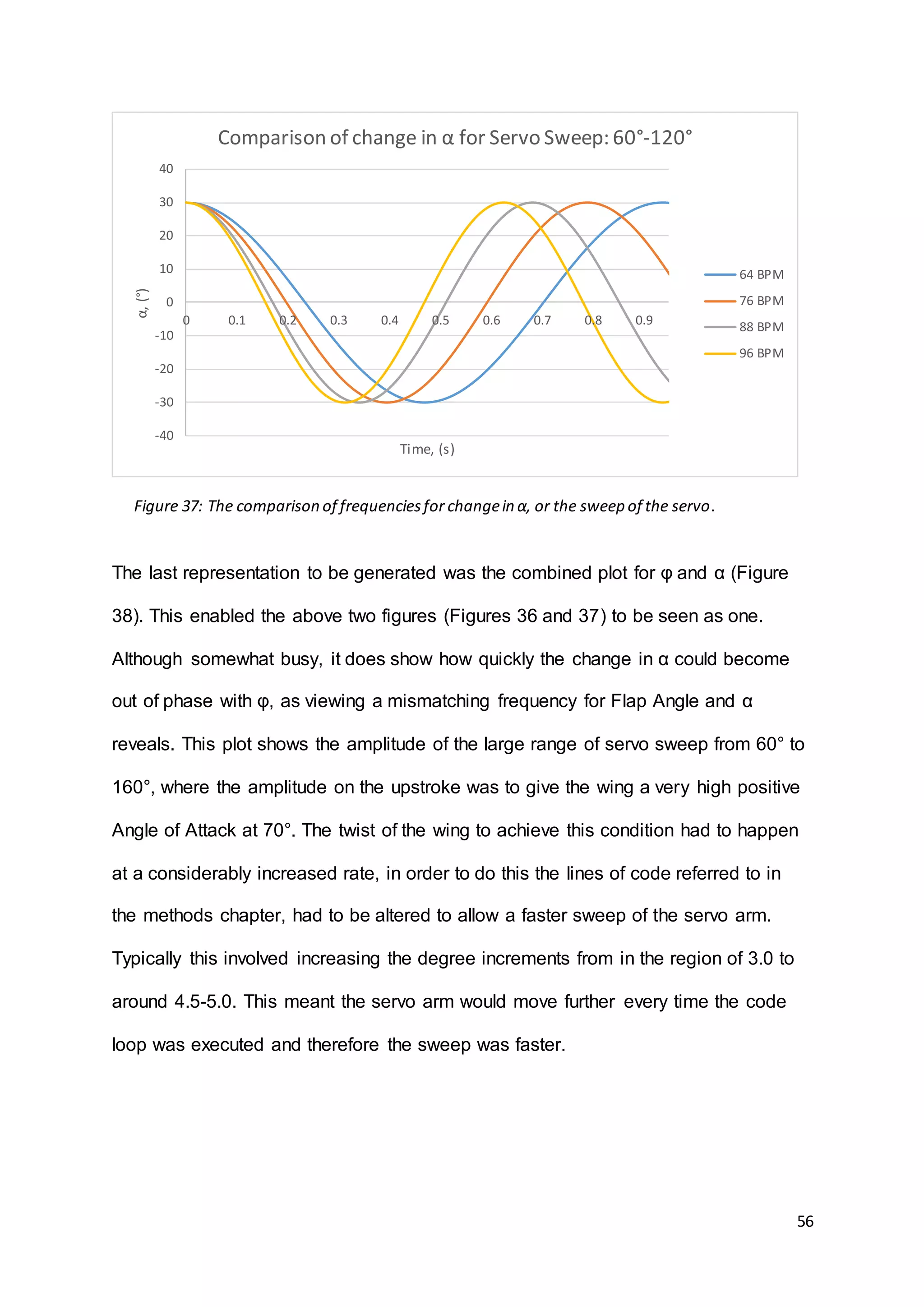
7.1.2. Component Flow Analysis
Applying the basic trigonometry for blade element theory, it was possible to predict
the effective angle of the flow felt by the wing [27]. Presented here in the results is
simply this resultant angle. It was found that as the free stream flow increased, the
angle of the resultant becomes increasingly smaller as can be seen in Figure 39.
These results prove the theory that in ‘zero’ velocity conditions, the test rig high
Angle of Attack on the upstroke would be important, especially at higher frequency.
Due to the low velocity which can be seen as the 1m/s line in Figure 39, we can see
the movement of the wing creates a large angle between the datum for the
freestream and the effective flow compared to faster flight speeds. This result would
also suggest that the test rig might benefit from further studies being carried out in a
wind tunnel, or some other form of freestream flow if future studies were to be made.
-40
-20
0
20
40
60
80
0 0.2 0.4 0.6 0.8 1
Angle(°)
Time, s
Relation between andφ and α for varying frequency (60-160)
64 BPM (Flap angle)
64 BPM (Alpha)
76 BPM (Flap angle)
76 BPM (Alpha)
88 BPM (Flap Angle)
88 BPM (Alpha)
96 BPM (Flap Angle)
96 BPM (Alpha)
Figure 38: A combined plot of φ and α fora rangeof -30° to +70° of wing twist.

58. 58
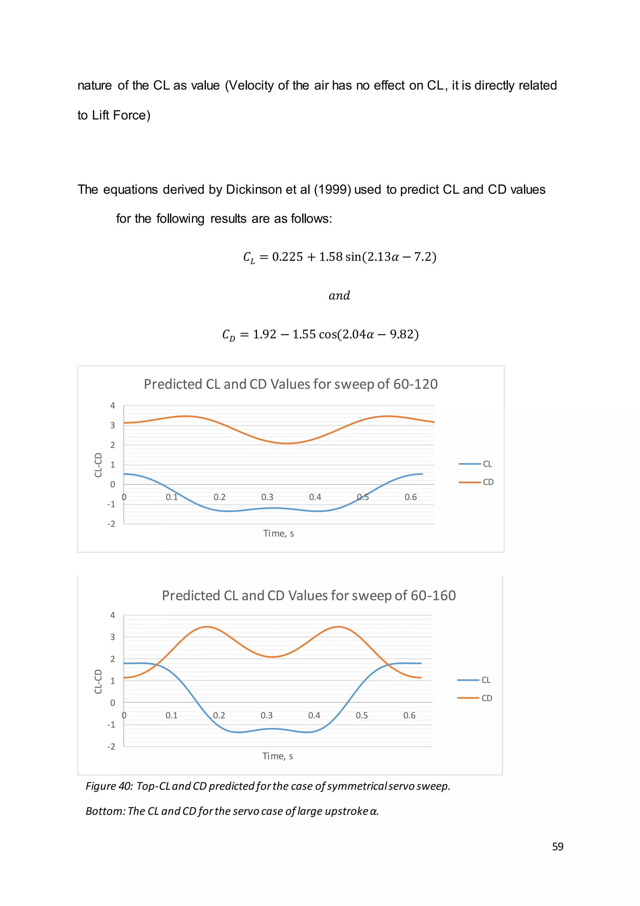
7.1.3. Lift Predictions Using Calculated CL Values
Using the method outlined by Sane and Dickinson (2001) [2] for their experimental
results, the same approach was taken with the calculated theoretical values obtained
for φ and α. This involved using equations derived by Dickinson et al (1999) [23] for
the approximation of CL and CD in flapping wings. Using this method, a separate
estimate of lifting force could be obtained to those found in XFLR5. Both approaches
would have their short comings, however both would provide results for comparison
to test results achieved. Figure 40 details the values found for both CL and CD for
both cases of the symmetrical ±30° α wing sweep, and the case of the wing having a
high α on the upstroke. These values would remain constant for any frequency (Also
the timescale plotted) over one period of the wings sinusoidal motion, due to the
0
10
20
30
40
50
60
5 15 25 35 45 55 65 75 85
Degrees°
Beats per Minute BPM
Beats per minute vs Resultant componentof flow over
wing.
@ 1 m/s
@ 2 m/s
@ 3 m/s
@ 4 m/s
@ 5 m/s
@ 6 m/s
@ 7 m/s
@ 8 m/s
@ 9 m/s
@ 10 m/s
Figure 39: The plotof theresultantflow anglestudy.Here theresultantα is shown on the
y axisagainstthebeatsper minute frequency of thewingsforvarying speedsof
freestreamflow.

59. 59
nature of the CL as value (Velocity of the air has no effect on CL, it is directly related
to Lift Force)
The equations derived by Dickinson et al (1999) used to predict CL and CD values
for the following results are as follows:
𝐶 𝐿 = 0.225 + 1.58 sin(2.13𝛼 − 7.2)
𝑎𝑛𝑑
𝐶 𝐷 = 1.92 − 1.55 cos(2.04𝛼 − 9.82)
-2
-1
0
1
2
3
4
0 0.1 0.2 0.3 0.4 0.5 0.6
CL-CD
Time, s
Predicted CL and CD Values for sweep of 60-120
CL
CD
-2
-1
0
1
2
3
4
0 0.1 0.2 0.3 0.4 0.5 0.6
CL-CD
Time, s
Predicted CL and CD Values for sweep of 60-160
CL
CD
Figure 40: Top-CLand CD predicted forthe case of symmetricalservo sweep.
Bottom:The CL and CD forthe servo case of large upstrokeα.

60. 60
Having found the CL of the wing, Lift Force could then be calculated using the lift equation.
This would produce a Lift Force plot for any wing case providing the velocity over the wing
was known. Figure 41 shows both Lift Force plots of the symmetrical and large upstroke α
cases at 96BPM as the CL is plotted in Figure 40.
7.1.4. Lift Force Predictions For The Wing Using XFLR5
By using XFLR5 it was possible to obtain a prediction of the wings CL throughout a
series of flight conditions. These CL values could then be used in the equation for
Lift Force to find the equivalent force produced by the wings. There were some
-1.5
-1
-0.5
0
0.5
1
1.5
2
0 0.1 0.2 0.3 0.4 0.5 0.6
ForceN
Time s
Predicted Lift Forcefor servo sweep: 60-120
Lift Force
-1.5
-1
-0.5
0
0.5
1
1.5
2
0 0.1 0.2 0.3 0.4 0.5 0.6
ForceN
Time, s
Predicted Lift Forcefor Servo Sweep: 60-160
Lift Force
Figure 41: Top- Lift Force predictionsforsymmetricalα sweep.
Bottom- Lift Forcepredictionsfor high α upstroke.

61. 61
limitations to carrying out this in XFLR5 as the software is primarily used for the
evaluation of fixed wing model aircraft, with no capacity to go into turbulent flow
conditions. This means it only has an accuracy at smaller angles of attack. It was not
practical to use different software or attempt to take this study any further, as trying
to model the wing Lift Force at higher angles of attack and in flapping conditions,
would be more than sufficient as work for a completely different project. This is due
to unsteady aerodynamic mechanisms being present around the wing during its
flapping motion that allow wings to stay effective beyond the normal point of stall. For
static conditions however, Figure 42 predicts the Lift Force that can be obtained with
change in Angle of Attack at varying freestream velocities. This would still be useful
as it enables an insight into the force that could be obtained by the wings if the twist
for Angle of Attack could be optimised. In the production of a flying vehicle this could
be invaluable when positioning the wing for both thrust and lift to keep the vehicle in
the air at constant velocity.

62. 62
7.1.5. XFLR5 Lift Force Predictions Across A Period Of Flapping
With all previous calculations made concerning Flap Angle and Angle of Attack,
Values of φ and α could be picked at time intervals through one period of flapping to
find the CL and Lift Force produced by the wings. This approach would allow a plot
for Lift Force of which values could be directly compared to the force obtained
experimentally from the load cell. There would be some limitations in doing this with
accuracy due to the previously mentioned downfalls of XFLR5. However along with
the plot of Lift Force against Angle of Attack, this provided the best approximation of
the performance expected.
The limitations of XFLR5 meant that the program could not model the CL of the wing
to a high Angle of Attack, however due to the resultant flow this was not completely
-6
-4
-2
0
2
4
6
8
10
12
-20 -15 -10 -5 0 5 10 15 20
LiftForceN
Angle of Attack (°)
Lift Force generated vs AOA across a range of
freestreamvelocities
1 m/s
2 m/s
3 m/s
4 m/s
5 m/s
6 m/s
7 m/s
8 m/s
9 m/s
Figure 42: The plotof theresults forAngle of attack,α vs Lift Force obtained fromthewings.The
forceobtained by the rig wasexpected to be in the lower region of Lift Force due to the static
natureof the testing,howeverit wasquite possiblethatmore forcemightbe obtained dueto the
unsteady mechanismsthatmay formon theflapping wings.

63. 63
necessary. As the resultant flow direction could be far from an α of 0°, this meant
that in reality the Angle of Attack of the flow experienced by the wing may not be as
great as the wing twist and could therefore be calculated by XFLR5. Because of this,
a reduction in α was assumed and the values scaled to be within the range of
XFLR5. Although not completely accurate, this would at least enable a prediction at
a flow velocity for incremental stages of a flapping cycle. All the values used for φ, α,
ρ and V were all taken from the previous stages of calculation.
Figure 43 shows an example of the initial prediction for Lift Force throughout a flap
cycle of the wings. This was made at a low frequency, as it was originally not known
how fast the mechanism would be capable of moving the wings without causing
damage. In reality this estimate was to low and the motor could not function properly
with the low revolutions required to flap the wings at 40 beats per minute. The Angle
of Attack was calculated as if the wings were flying at 3m/s freestream velocity to be
at an Angle of Attack of 7° for the best Lift/Drag ratio.
0
1
2
3
4
5
6
7
8
9
0 0.15 0.3 0.45 0.6 0.75 0.9 1.05 1.2 1.35 1.5
LiftForce(N)
Time (s)
Lift Forcevs Time @40 BPM (Sweep: -4°to 10°)
1m/s
2m/s
3m/s
4m/s
5m/s
6m/s
7m/s
8m/s
9m/s
Figure 43: A plot of Lift Forceover a flap cycle for 40 Beatsper minute with a sweep of
the wing twist between -4° and 10°.

64. 64
The same process to obtain results was undertaken for some specific cases of
flapping configuration. One of these cases was for the wing at a frequency of
96BPM, with a wing twist for an α of -30° to 70°. This Angle of Attack was not
possible in XFLR5, however as previously mentioned, due to resultant flow, in reality
the wing would not be achieving the high value of 70° due to the resultant angle of
the velocity component. Instead the maximum possible values for the aerofoil were
used at +30° and -20°. These were then mapped and scaled to the range of the wing
twist that would be applied for the experimental test. This should provide a result that
although was not directly comparable, did give an indication of a calculated force.
The plot in Figure 44 shows that for the low velocity cases, a lifting force of 1N or
less was to be expected from the wings. This estimate seemed a reasonable value
to expect from physical testing, as once the test rig had built up to speed, and the
wings were flapping, it would be reasonable to assume that there would be some
airflow around them. For an idea of the numerical value of the forces calculated from
this same example, the table of values used for the plot of the 1, 2 and 3m/s cases is
shown in Figure 45.
-10
-5
0
5
10
15
20
0 0.15 0.3 0.45 0.6
LiftForce(N)
Time (s)
Lift Forcevs Time @96BPM(Sweep: -20°to 30°)
1 m/s
2 m/s
3m/s
4m/s
5 m/s
6 m/s
7 m/s
8 m/s
9 m/s
10 m/s
Figure 44: The Lift
Force vstime plotfor
the calculated
numericalanalysis
with thelargest
possibleangleof
attackpossiblein
XFLR5 applied.

65. 65
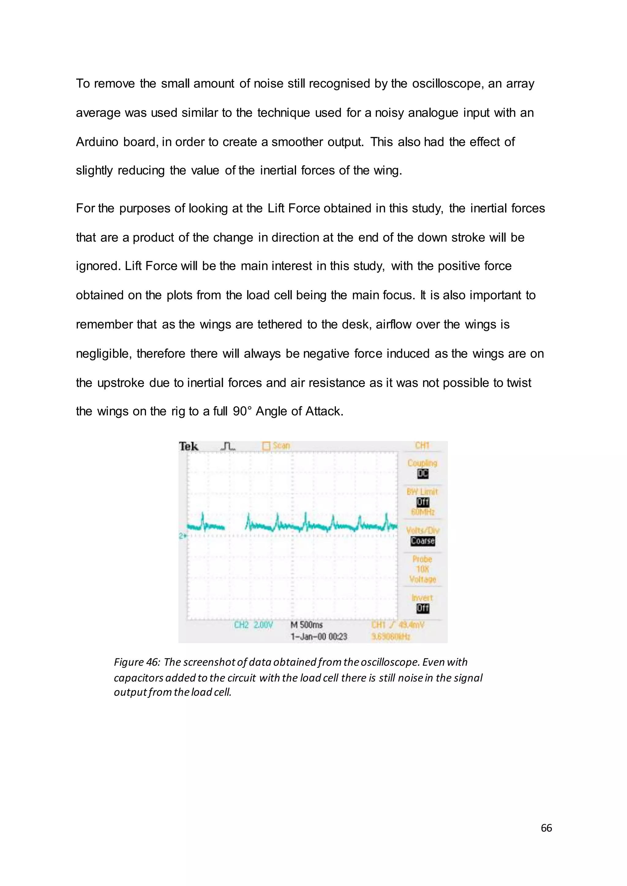
7.2. ExperimentalResults
The results obtained from the load cell on the test rig were the product of a snapshot
taken from the oscilloscope screen. This meant that the results initially covered a
series of flap cycles and still contained some noise, even though capacitors had
been added to the circuit across the output leads to quieten the signal. An example
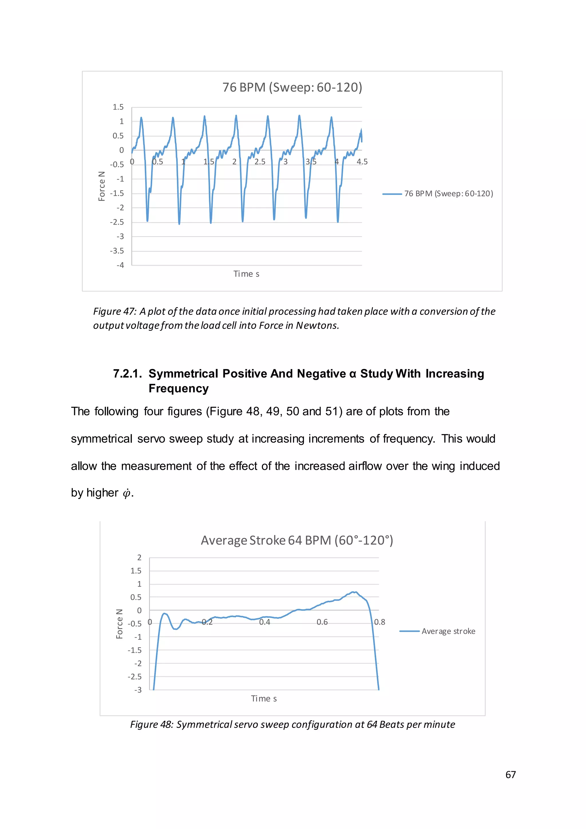
of a screen shot from the oscilloscope can be seen in Figure 46 with Figure 47 being
a plot of the force obtained after initial averaging and manipulation of the raw
numerical data. It would not be useful to analyse the results of multiple wing flaps as
some inconsistency could be found, it would also be hard to compare the large
amount of data generated over two cases. Because of this it was decided that the
best approach was that of Sane and Dickinson (2001) [2], where the average of
multiple wing strokes was taken to provide data for just a single wingbeat. This would
lead to any anomalies being lost into a data set for a single wing beat of averages.
Time φ α CL
Force @1
m/s (N)
Force
@2 m/s
(N)
Force
3m/s
(N)
0 0 30 1.69 0.144918 0.57967 1.304258
0.0694 13.81 22.98 1.4623 0.125392 0.501569 1.12853
0.104 19.26 15 1.2976 0.111269 0.445077 1.001423
0.16 21.17 0 0.3493 0.029952 0.11981 0.269572
0.226 16.5 -19.28 -0.77 -0.06603 -0.26411 -0.59425
0.3125 0 -30 -0.834 -0.07152 -0.28606 -0.64364
0.43 -21.17 -10.26 -0.0014 -0.00012 -0.00048 -0.00108
0.469 -21.5 0 0.3483 0.029867 0.119467 0.268801
0.556 -13.82 23 1.4608 0.125264 0.501054 1.127372
0.59 -10.5 28.19 1.6763 0.143743 0.574971 1.293685
Figure 45: The tableof numericalvaluesshowing thepredicted forces forfigure10. Valuesof 1.3N at
peaklifting forcewould be good to obtain experimentally and show thatthedesign of thetest rig could
be feasible.

66. 66
To remove the small amount of noise still recognised by the oscilloscope, an array
average was used similar to the technique used for a noisy analogue input with an
Arduino board, in order to create a smoother output. This also had the effect of
slightly reducing the value of the inertial forces of the wing.
For the purposes of looking at the Lift Force obtained in this study, the inertial forces
that are a product of the change in direction at the end of the down stroke will be
ignored. Lift Force will be the main interest in this study, with the positive force
obtained on the plots from the load cell being the main focus. It is also important to
remember that as the wings are tethered to the desk, airflow over the wings is
negligible, therefore there will always be negative force induced as the wings are on
the upstroke due to inertial forces and air resistance as it was not possible to twist
the wings on the rig to a full 90° Angle of Attack.
Figure 46: The screenshotof data obtained fromtheoscilloscope.Even with
capacitorsadded to the circuit with the load cell there is still noisein the signal
outputfromtheload cell.

67. 67
7.2.1. Symmetrical Positive And Negative α Study With Increasing
Frequency
The following four figures (Figure 48, 49, 50 and 51) are of plots from the
symmetrical servo sweep study at increasing increments of frequency. This would
allow the measurement of the effect of the increased airflow over the wing induced
by higher 𝜑̇.
-4
-3.5
-3
-2.5
-2
-1.5
-1
-0.5
0
0.5
1
1.5
0 0.5 1 1.5 2 2.5 3 3.5 4 4.5
ForceN
Time s
76 BPM (Sweep: 60-120)
76 BPM (Sweep:60-120)
-3
-2.5
-2
-1.5
-1
-0.5
0
0.5
1
1.5
2
0 0.2 0.4 0.6 0.8
ForceN
Time s
AverageStroke64 BPM (60°-120°)
Average stroke
Figure 47: A plot of the dataonce initial processing had taken place with a conversion of the
outputvoltagefromtheload cell into Force in Newtons.
Figure 48: Symmetrical servo sweep configuration at 64 Beats per minute

68. 68
-3
-2.5
-2
-1.5
-1
-0.5
0
0.5
1
1.5
2
0 0.1 0.2 0.3 0.4 0.5 0.6
ForceN
Time s
AverageStroke76 BPM (Sweep: 60°-120°)
Average Stroke
-3
-2.5
-2
-1.5
-1
-0.5
0
0.5
1
1.5
2
0 0.1 0.2 0.3 0.4 0.5 0.6
ForceN
Time s
AverageStroke88BPM(60°-120°)
Average Stroke
-3
-2.5
-2
-1.5
-1
-0.5
0
0.5
1
1.5
2
0 0.1 0.2 0.3 0.4 0.5 0.6
ForceN
Time s
AverageStroke96 BPM (Sweep: 60°-120°)
Average Stroke
Figure 49: Symmetrical servo sweep configuration at 76 Beats per minute
Figure 50: Symmetricalservo sweep configuration at88 Beats per minute
Figure 51: Symmetrical servo sweep configuration at 96 Beats per minute

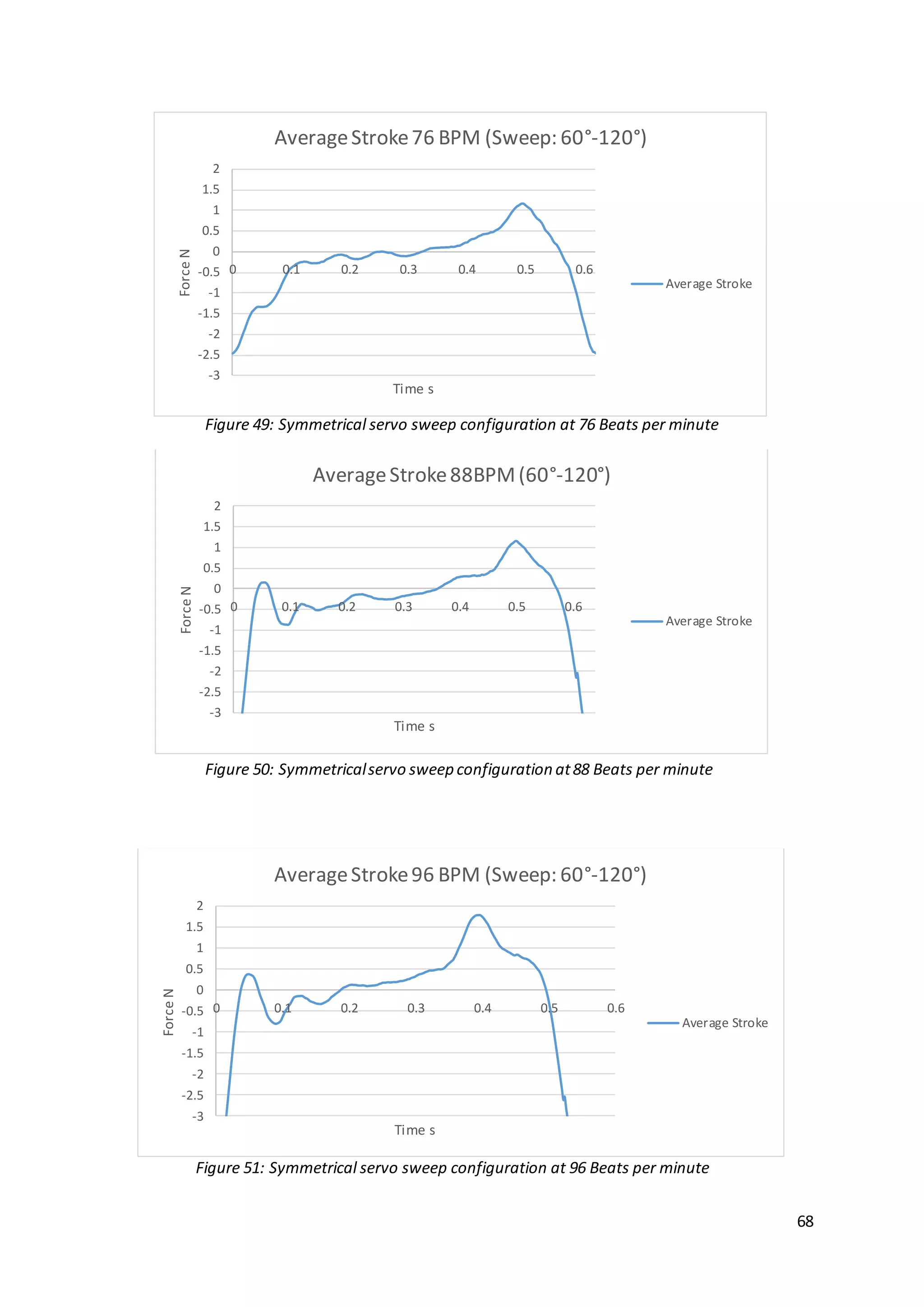
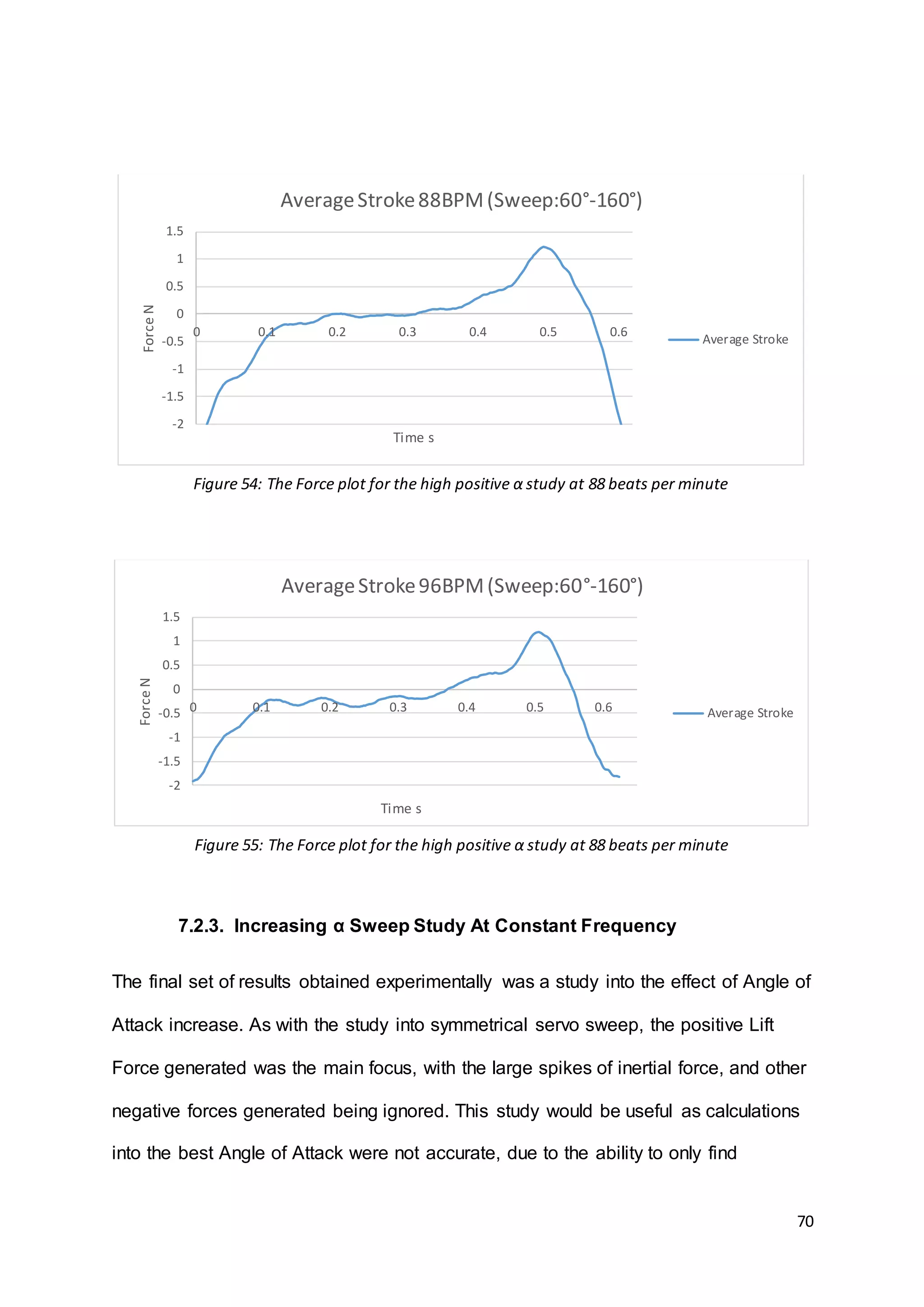
69. 69
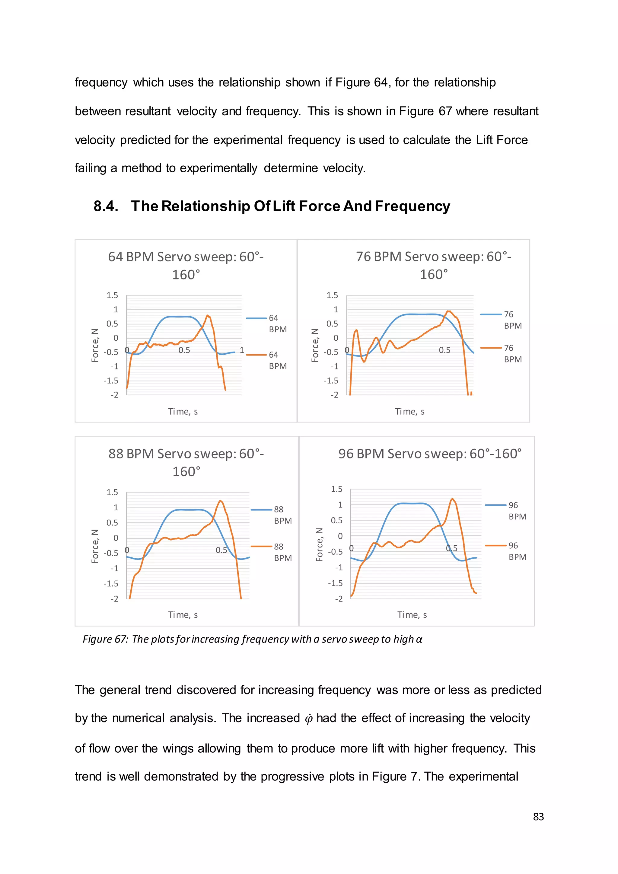
7.2.2. High Positive α Study With Increasing Frequency
The next study made was again into the increasing frequency of flapping, but with
the variation of a much higher Angle of Attack on the upstroke. As mentioned by
Anderson (2001), the rapid pitch up at the end of the stroke allows higher CL to be
achieved towards the end of the lift stroke [20]. The higher α in the upstroke should
also produce less negative force due to the reduced surface area perpendicular to
the velocity of the wings centre of mass. The results for this study are plotted in
Figures 52, 53, 54 and 55. All increments in the increase in frequency have been
kept the same as for the symmetrical servo sweep study.
-2
-1.5
-1
-0.5
0
0.5
1
1.5
0 0.2 0.4 0.6 0.8
ForceN
Time s
AverageStroke64 BPM (Sweep:60°-160°)
Average Stroke
-2
-1.5
-1
-0.5
0
0.5
1
1.5
0 0.1 0.2 0.3 0.4 0.5 0.6
ForceN
Time s
AverageStroke76 BPM (Sweep:60°-160°)
Average Stroke
Figure 52: The Force plot for the high positive α study at 64 beats per minute
Figure 53: The Force plot for the high positive α study at 76 beats per minute

70. 70
7.2.3. Increasing α Sweep Study At Constant Frequency
The final set of results obtained experimentally was a study into the effect of Angle of
Attack increase. As with the study into symmetrical servo sweep, the positive Lift
Force generated was the main focus, with the large spikes of inertial force, and other
negative forces generated being ignored. This study would be useful as calculations
into the best Angle of Attack were not accurate, due to the ability to only find
-2
-1.5
-1
-0.5
0
0.5
1
1.5
0 0.1 0.2 0.3 0.4 0.5 0.6
ForceN
Time s
AverageStroke88BPM(Sweep:60°-160°)
Average Stroke
-2
-1.5
-1
-0.5
0
0.5
1
1.5
0 0.1 0.2 0.3 0.4 0.5 0.6
ForceN
Time s
AverageStroke96BPM(Sweep:60°-160°)
Average Stroke
Figure 54: The Force plot for the high positive α study at 88 beats per minute
Figure 55: The Force plot for the high positive α study at 88 beats per minute

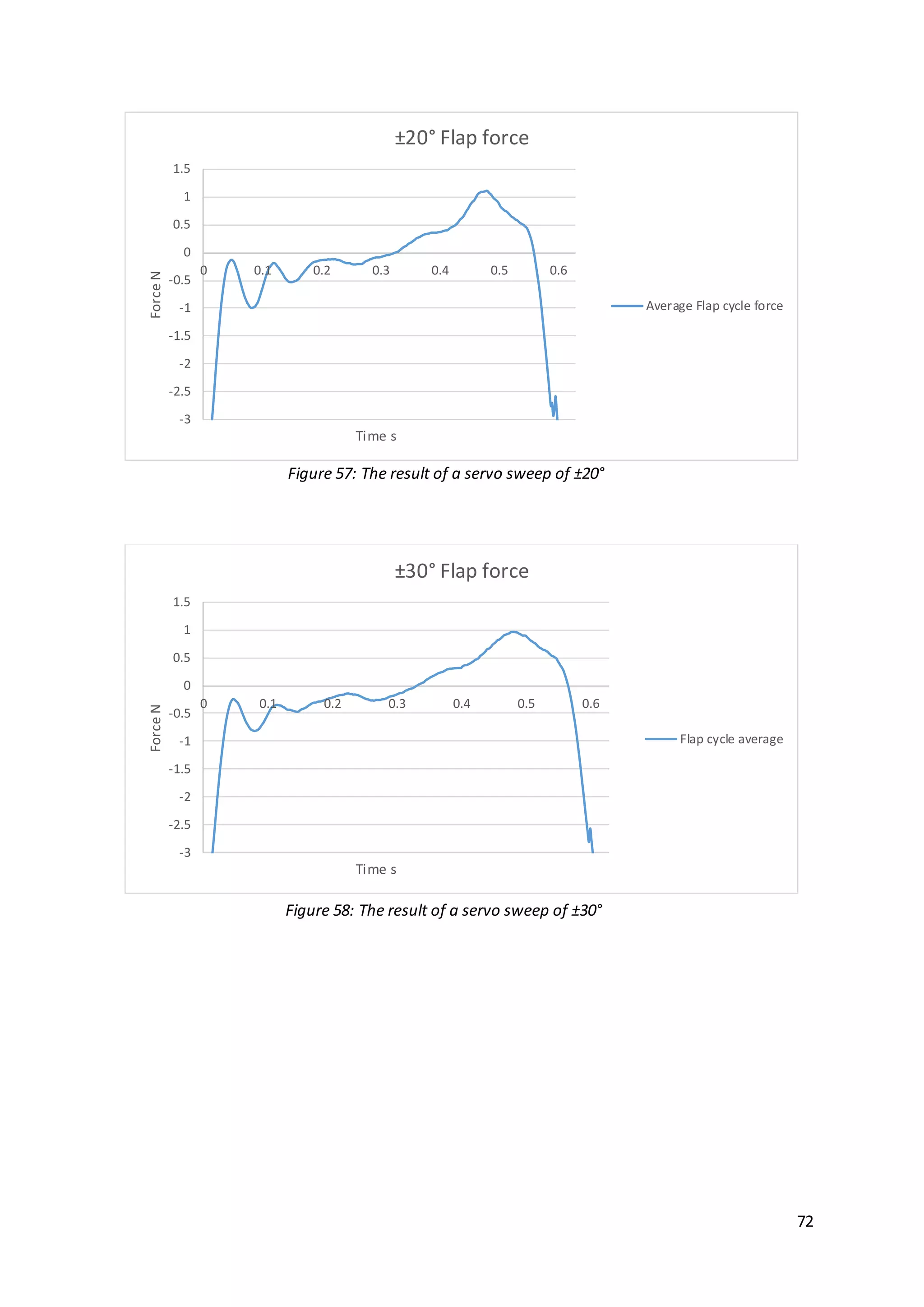
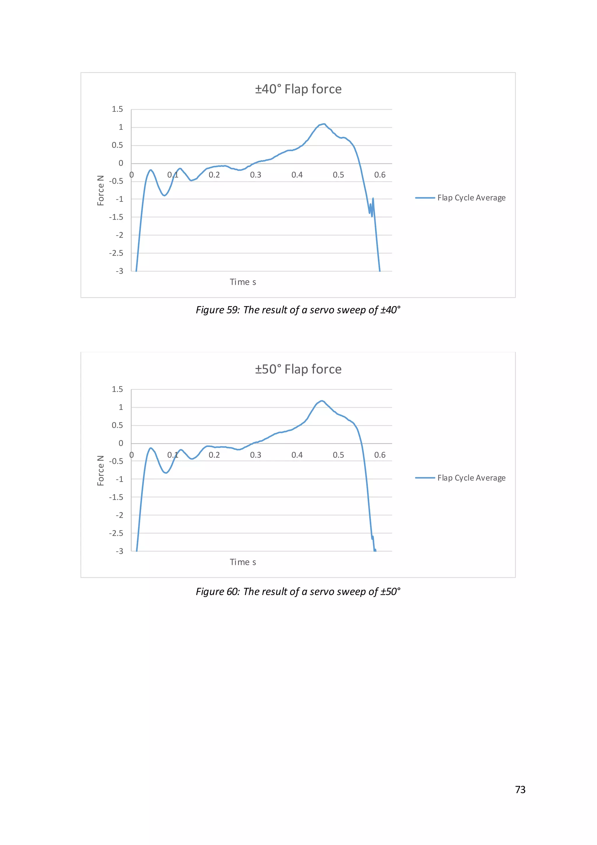
71. 71
solutions to a static wing in two dimensional flow. The case of flapping would present
a far more difficult problem and for the purposes of this project would be better
analysed experimentally. The symmetrical servo sweep analysed, ranged from ±10°
through to ±50° in increments of 10°. These results are shown in Figure 56 to 60.
The same procedure was used as for the previous results by applying Sane and
Dickinson’s method [2] of averaging all strokes measured into a single wing beat.
This would keep all results obtained consistent.
-3
-2.5
-2
-1.5
-1
-0.5
0
0.5
1
1.5
0 0.1 0.2 0.3 0.4 0.5 0.6
ForceN
Time s
±10° Flap force
Flap cycle average
Figure 56: The result of a servo sweep of ±10°

72. 72
-3
-2.5
-2
-1.5
-1
-0.5
0
0.5
1
1.5
0 0.1 0.2 0.3 0.4 0.5 0.6
ForceN
Time s
±20° Flap force
Average Flap cycle force
-3
-2.5
-2
-1.5
-1
-0.5
0
0.5
1
1.5
0 0.1 0.2 0.3 0.4 0.5 0.6
ForceN
Time s
±30° Flap force
Flap cycle average
Figure 57: The result of a servo sweep of ±20°
Figure 58: The result of a servo sweep of ±30°

73. 73
-3
-2.5
-2
-1.5
-1
-0.5
0
0.5
1
1.5
0 0.1 0.2 0.3 0.4 0.5 0.6
ForceN
Time s
±40° Flap force
Flap Cycle Average
-3
-2.5
-2
-1.5
-1
-0.5
0
0.5
1
1.5
0 0.1 0.2 0.3 0.4 0.5 0.6
ForceN
Time s
±50° Flap force
Flap Cycle Average
Figure 59: The result of a servo sweep of ±40°
Figure 60: The result of a servo sweep of ±50°

74. 74
8. Chapter 3: Analysis
The results for the numerical modelling and the experimental studies allowed a
comparison between the theoretical calculations and reality. Not only would these
comparisons provide answers, but the differences between the experimental results
and the theory proved to be just as revealing as the similarities as to the challenges
of flapping wing flight. As well as considerations that would need to be made or
addressed in the design of an MAV. These answers or new challenges would not
only come from the results but also from the design and operation of the test rig,
revealing design faults that may have already been addressed by the designers of
previous successful projects such as the Festo Smartbird[3].
8.1. The Design
The selection of wood as the predominant material was chosen because of the
speed in producing parts by laser cutting. However this added unnecessary weight to
the test rig. The 3mm and 5mm thick plywood used is the same as that used in
remote control model aeroplanes. However these thicknesses were more than
required as the structure proved plenty strong enough. As to the loads induced on
the wood, the design played well to the material strengths, adding to the case for the
potential of thinner wood. Alternatively, the ribs could have been made from much
lighter balsa wood due to the loads being quite low and the structure more than
adequate.
Looking at the results of experimental testing, the most noticeable characteristic is
the large peak of negative force. This is created by the large inertial forces produced
by the wings, as their momentum is rapidly damped at the end of each downstroke.
This is amplified by the motion of the mechanism quickly lifting the wings for the

75. 75
upstroke. The use of carbon fibre in the Festo Smartbird, allows for a lightweight,
tough design that can withstand harder landings. Furthermore, the Smartbird’s two
part wing may have corrected the problem of large negative inertial forces. The out
of phase movement of the wings in the Smartbird could reduce momentum by
always having one of both panels of the wing moving while the other is stationary. In
comparison to the test rig, which has an aggressive flapping style, this provides a
much smoother flap cycle.
The second design point of interest was the use of the servos for wing twist. On the
Smartbird, these are located towards the tip of the wing, in line with the spar that the
wing rotates around. Although the connection of the servo arm to a sliding pin in the
wing hinge did prove effective, in an improved version of the test rig, this would be a
point for a major redesign. In testing the end of the pin would be jammed by the test
rig frame at the extremes of φ, the distance between the servo arm and the sliding
pin track also proved problematic with moments causing some bending. The
configuration of the servo connected directly to the spar instantly overcomes these
problems, and although space is limited at the tip of the test rig wings, there is no
reason why the solution could not be implemented at the centre of the wing (Figure
61). If the current mechanism was kept in an improved version, it is likely a metal
servo arm would be needed for strength with a better fixing to the pin. A different
material would also be needed for the sliding pin track, as the 3D printed plastic was
quick to wear.

76. 76
Another key area of improvement was the fixing of the push rod gears to the frame. These
gears were constantly brought out of line by the load of the wings through the push rod, this
was improved by gluing the washers that held them in place closer to the frame. However
the issue still remained (Figure 62). In all other projects, similar mechanisms are used with
pushrods on circular gears, with gears remaining in the correct plane. An improved version
would seek to learn more from previous projects, and how the gears were fixed. This may be
that the tolerances are much finer for a tighter fit of the axel to the frame, or potentially an
improved version may use the method of keeping the axel fixed in position with the gear
rotating around it.
Figure 61: The Dashed red box shows the potential location of the servo in a redesign.

77. 77
8.2. Flap Angle, φ And Angle Of Attack, α
The flap angle and alpha calculations in the numerical analysis proved hard to
implement in the physical model of the test rig. Without a feedback or sensor
connected to the Arduino to measure the rate of change of φ, it was hard to properly
synchronise the twist of the servos. This meant that considerable calibration had to
be done before the running of any test in order to find values that produced the
correct amount of cycles per minute, from both the servos and motor individually.
Once inputs were found to give an approximate timing, the servos and motor were
run together and fine-tuned to be synchronised. This however was still not a
complete solution, as it would be impossible to know the precise φ in order to induce
an appropriate twist for the desired α.
Figure 62: The two red gearsside by side had problemswith alignment.Thiswasmainly down to
the large toleranceof the holes in the framefortheir axels.Fixing the axelsto the frameand
allowing the gearsto rotatearound themmay havebeen a betterconfiguration fortheload
carrying gears.

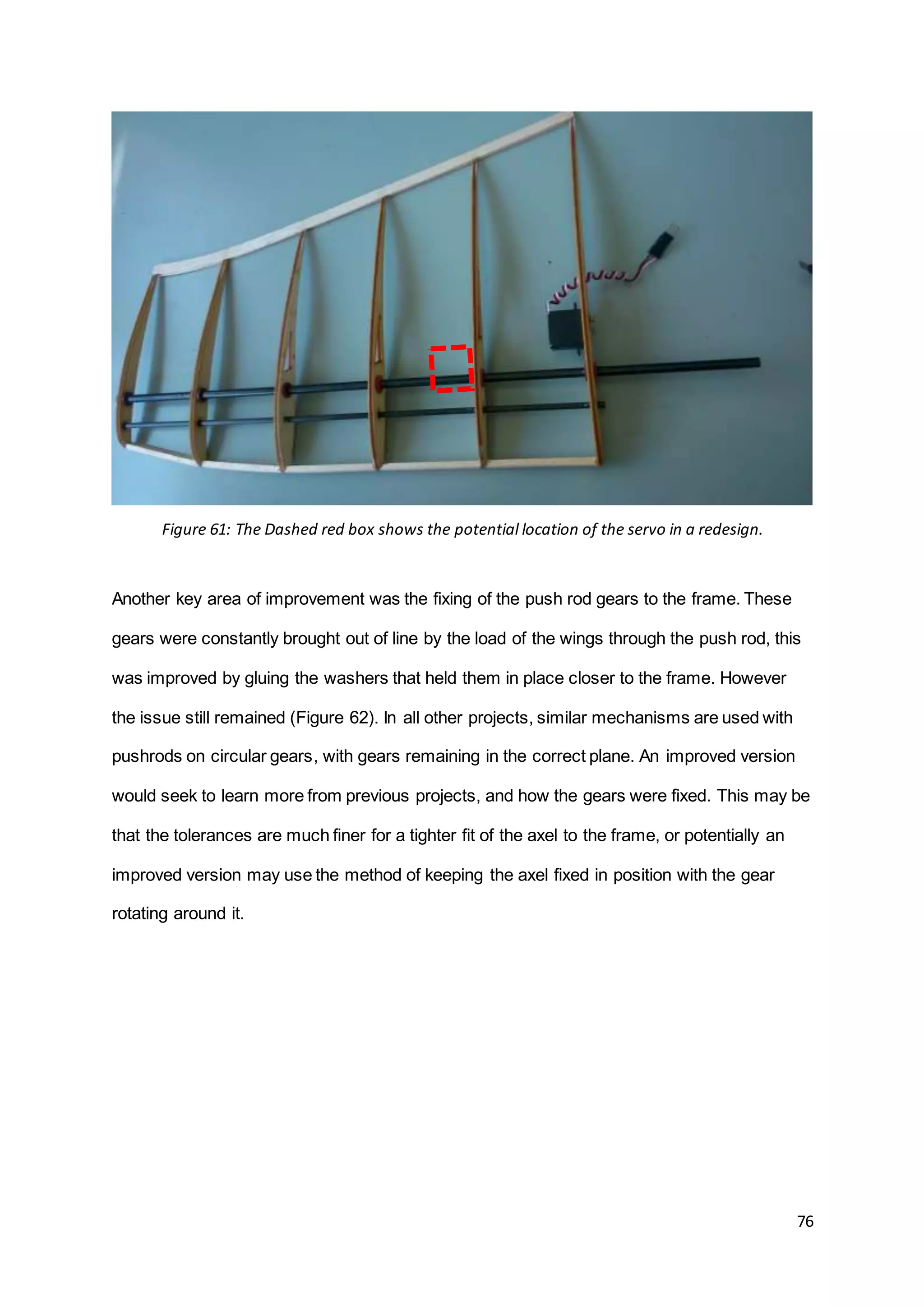
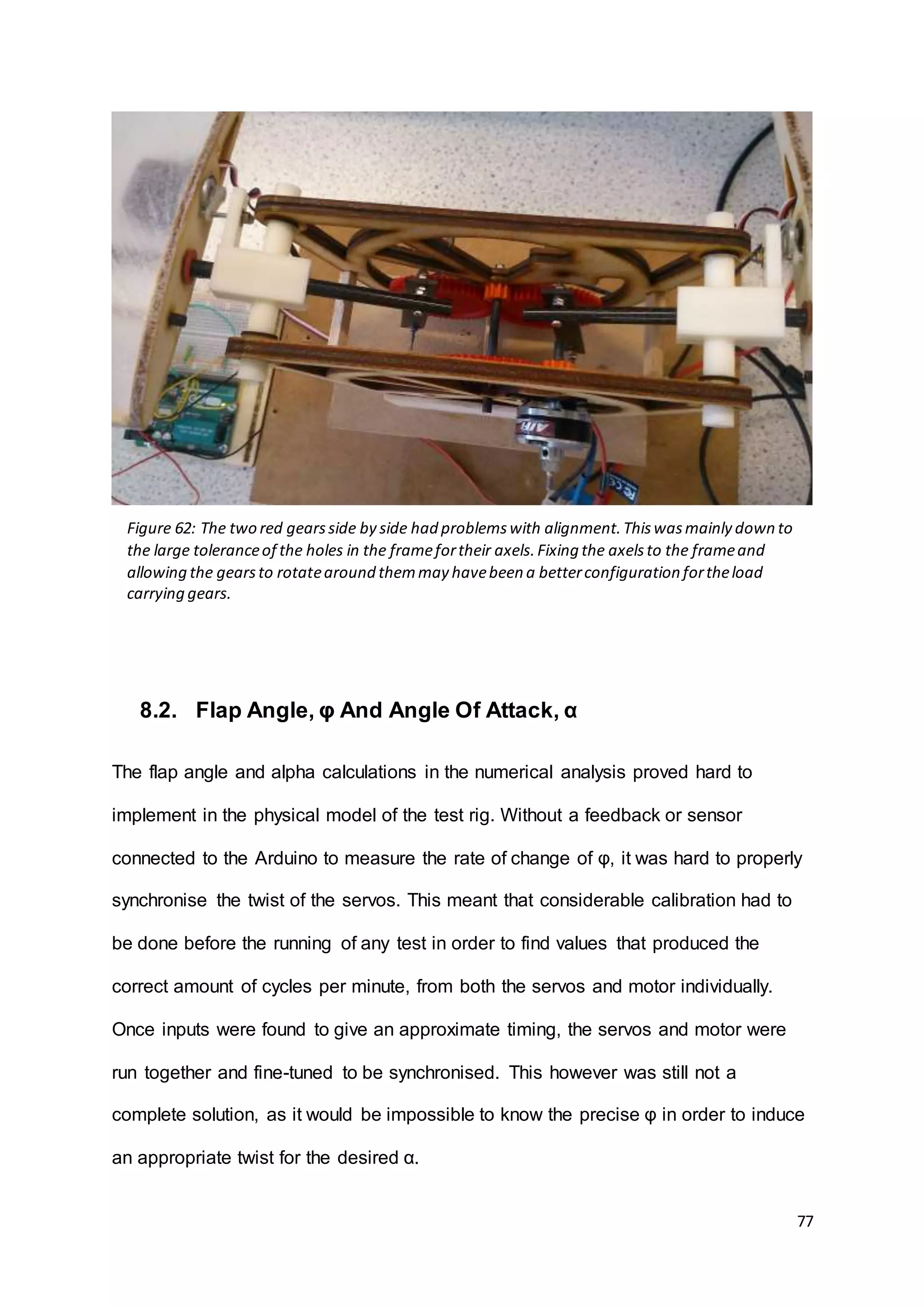
78. 78
With further work on the project, the addition of sensors would be the most practical
and useful modification. A sensor could easily be positioned on the frame to register
the movement of one of the gears or the wing spar. This could be used as a trigger
to activate a twist of the servo with regard to its current position. This addition would
alleviate the need for calibration and the correct starting position of the test rig,
allowing the parameters affecting beats per minute to be changed exclusively with
the speed of the motor.
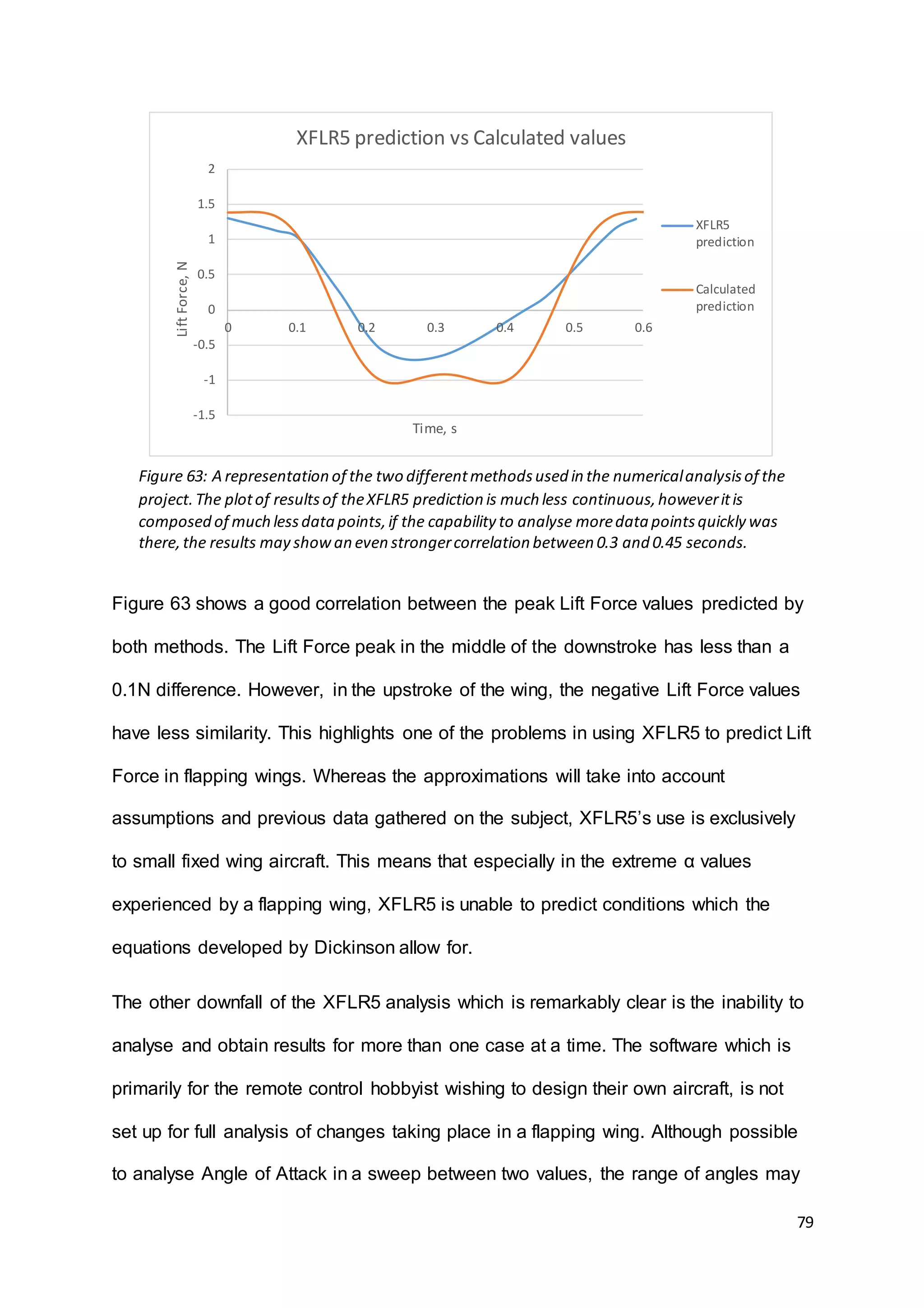
8.3. Comparisons Between The Lift Force Calculated And Lift
Force Determined Experimentally.
Due to the nature of the numerical analysis, it was possible to use two different
methods for calculating the Lift Force produced by the wings. One method would
apply the calculation of sinusoidal functions of φ and α as by Whitney and Wood
(2012) [22], to then apply equations for the approximation of CL and CD as by
Dickinson et al (1999) [23] to finally produce a force prediction from the lift equation.
The second method for theoretically determining the lift would again use calculation
of φ and α to then run an analysis on increments of the flap cycle in XFLR5 to find a
CL, this would then as before, be used in the lift equation. Both methods would have
their advantages and disadvantages but when comparing the two methods over a
single case with identical values of φ, α, 𝑉∞ and ρ, there is a strong correlation
between the results obtained. A comparison is shown in Figure 63 with a comparison
between the methods for a case of 96BPM, an Angle of Attack sweep of -30° to
+70°, and a freestream velocity of 3m/s.

79. 79
Figure 63 shows a good correlation between the peak Lift Force values predicted by
both methods. The Lift Force peak in the middle of the downstroke has less than a
0.1N difference. However, in the upstroke of the wing, the negative Lift Force values
have less similarity. This highlights one of the problems in using XFLR5 to predict Lift
Force in flapping wings. Whereas the approximations will take into account
assumptions and previous data gathered on the subject, XFLR5’s use is exclusively
to small fixed wing aircraft. This means that especially in the extreme α values
experienced by a flapping wing, XFLR5 is unable to predict conditions which the
equations developed by Dickinson allow for.
The other downfall of the XFLR5 analysis which is remarkably clear is the inability to
analyse and obtain results for more than one case at a time. The software which is
primarily for the remote control hobbyist wishing to design their own aircraft, is not
set up for full analysis of changes taking place in a flapping wing. Although possible
to analyse Angle of Attack in a sweep between two values, the range of angles may
-1.5
-1
-0.5
0
0.5
1
1.5
2
0 0.1 0.2 0.3 0.4 0.5 0.6
LiftForce,N
Time, s
XFLR5 prediction vs Calculated values
XFLR5
prediction
Calculated
prediction
Figure 63: A representation of the two differentmethodsused in the numericalanalysisof the
project.The plotof resultsof theXFLR5 prediction is much less continuous,howeveritis
composed of much lessdatapoints,if the capability to analyse moredata pointsquickly was
there,the results may showan even strongercorrelation between 0.3 and 0.45 seconds.

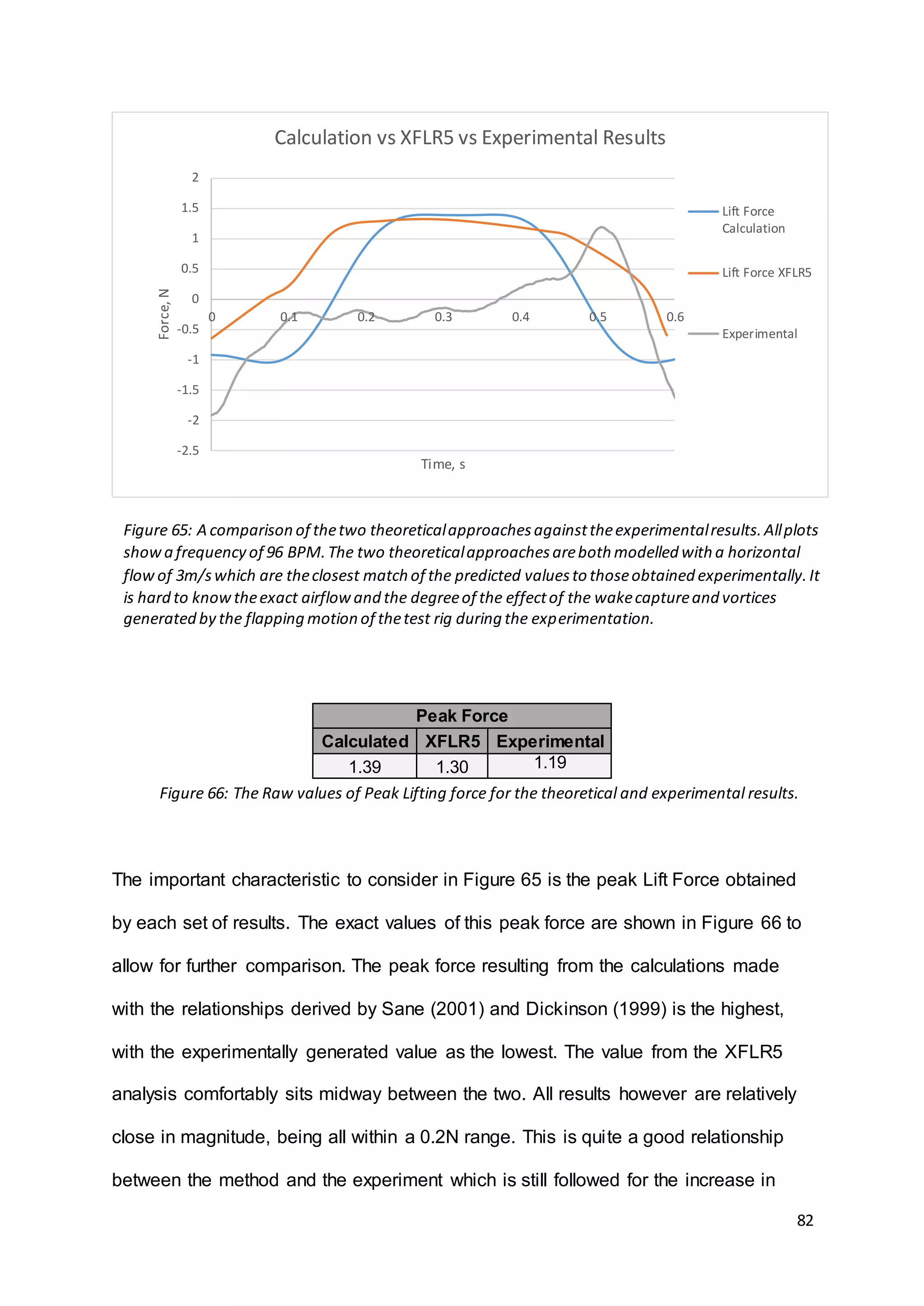
80. 80
only span across a maximum of 40° at a time. The software is also able to do the
same with freestream velocity. However in the example of a flapping wing vehicle,
the software cannot sweep through more than one set of parameters at a time, and
in the case of wing dihedral which is constantly changing in flapping flight, this must
be altered manually every time. To this end, the plot of the XFLR5 results is
composed of only 10 data points, with plots for the calculated values containing
some 37 data points. This becomes obvious when viewing them side by side, as the
plot for the XFLR5 values is far less continuous in profile due to a far less regular
spacing of values. This is not to say however, that an XFLR5 analysis with more data
points could provide a much more coherent analysis.
Figure 64 shows the predicted increase in the freestream flow over its value due to
the added component of the wings velocity in the downstroke. From the results of the
application of blade element theory, which treats the wing as a propeller blade
moving at a constant velocity perpendicular to an oncoming flow, it can be seen that
the increase becomes less with increasing horizontal airspeed. An airspeed of 1m/s
0
0.5
1
1.5
2
2.5
3
3.5
0 20 40 60 80 100
Velocity,m/s
Frequency BPM
Low Speed resultantvelocity induced by flapping
@ 1 m/s
@ 2 m/s
@ 3 m/s
Figure 64: The predictions for low velocity resultant flow over the wings using Blade element
theory [27].

81. 81
sees an increase of almost 100% with a frequency of 90BPM. However at the same
frequency, a freestream flow of 3m/s experiences only around a 33% increase.
Interestingly, when it comes to the experimental setup, these theoretical calculations
would suggest that the test rig experiences a significant induced horizontal flow from
its own motion. The force calculations made at 3m/s produce peak Lift Force values
similar in magnitude to those seen from the experimental results, most notably those
in Figure 54 and 55 (In Chapter 2) for 88BPM and 96 BPM with large servo sweep. A
comparison of theoretical against the experimental results for the same case is seen
in Figure 65. This would suggest that either the flow experienced by the wings after
run up to the correct speed was considerably higher than predicted, or that in reality
the unsteady aerodynamic mechanisms present in flapping wings are responsible for
a large portion of lift generated at stationary conditions. However it is also possible
that the flow associated with the vortices is created by the unsteady mechanisms
responsible for the increase, as is the possibility of the wake of previous wing strokes
having an effect of airflow.
The solution to the increased Lift Force over that expected is not entirely certain. The
lack of flow visualisation, control over horizontal flow and local air conditions, or any
sensors to determine pressure around the wing make finding the solution to this very
difficult. In further work, these criteria would make for an interesting investigation and
help to further validate experimental results. Some indications however prove that
flows were certainly created by the running test rig, such as movement of small loose
debris on the desk.

82. 82
The important characteristic to consider in Figure 65 is the peak Lift Force obtained
by each set of results. The exact values of this peak force are shown in Figure 66 to
allow for further comparison. The peak force resulting from the calculations made
with the relationships derived by Sane (2001) and Dickinson (1999) is the highest,
with the experimentally generated value as the lowest. The value from the XFLR5
analysis comfortably sits midway between the two. All results however are relatively
close in magnitude, being all within a 0.2N range. This is quite a good relationship
between the method and the experiment which is still followed for the increase in
-2.5
-2
-1.5
-1
-0.5
0
0.5
1
1.5
2
0 0.1 0.2 0.3 0.4 0.5 0.6
Force,N
Time, s
Calculation vs XFLR5 vs Experimental Results
Lift Force
Calculation
Lift Force XFLR5
Experimental
Peak Force
Calculated XFLR5 Experimental
1.39 1.30 1.19
Figure 65: A comparison of thetwo theoreticalapproachesagainsttheexperimentalresults.Allplots
showa frequency of 96 BPM.The two theoreticalapproachesareboth modelled with a horizontal
flow of 3m/swhich are theclosest match of the predicted valuesto thoseobtained experimentally.It
is hard to knowtheexact airflowand the degreeof the effectof the wakecaptureand vortices
generated by the flapping motion of thetest rig during the experimentation.
Figure 66: The Raw values of Peak Lifting force for the theoretical and experimental results.

83. 83
frequency which uses the relationship shown if Figure 64, for the relationship
between resultant velocity and frequency. This is shown in Figure 67 where resultant
velocity predicted for the experimental frequency is used to calculate the Lift Force
failing a method to experimentally determine velocity.
8.4. The Relationship OfLift Force And Frequency
The general trend discovered for increasing frequency was more or less as predicted
by the numerical analysis. The increased 𝜑̇ had the effect of increasing the velocity
of flow over the wings allowing them to produce more lift with higher frequency. This
trend is well demonstrated by the progressive plots in Figure 7. The experimental
-2
-1.5
-1
-0.5
0
0.5
1
1.5
0 0.5 1
Force,N
Time, s
64 BPM Servo sweep: 60°-
160°
64
BPM
64
BPM
-2
-1.5
-1
-0.5
0
0.5
1
1.5
0 0.5
Force,N
Time, s
76 BPM Servo sweep: 60°-
160°
76
BPM
76
BPM
-2
-1.5
-1
-0.5
0
0.5
1
1.5
0 0.5
Force,N
Time, s
88 BPM Servo sweep: 60°-
160°
88
BPM
88
BPM
-2
-1.5
-1
-0.5
0
0.5
1
1.5
0 0.5
Force,N
Time, s
96 BPM Servo sweep: 60°-160°
96
BPM
96
BPM
Figure 67: The plotsforincreasing frequency with a servo sweep to high α

84. 84
force is obtained using the predicted flow increase with frequency for a horizontal
component of 2m/s. This relationship can be found in Figure 64 and is used as a
representation of aerodynamic mechanisms that are likely to be in action around the
wing, as before measuring, the wings were run up to the frequency under
investigation.
This trend was shown far more exaggerated in the study for increasing frequency
with symmetrical servo sweep. Looking at the experimental results for the peak
positive lifting force between Figure 48 and Figure 51(Chapter 2), there is a
difference of around 1N of lifting force. Here the maximum positive Lift Force
achieved by the test rig at 96BPM is 1.78N, considerably higher than that achieved
with the high α upstroke configuration of flapping. This is likely down to the time it
takes the wing servos to carry out their sweep for the change of the wings Angle of
Attack. The quicker movement of the servo arm needed for the high alpha upstroke
may cause one of two problems: the first may be that the faster travel of the servo
leaves the wing with less time in the downstroke close to its optimum Angle of
Attack. The second may be that the asymmetrical wing twist between positive and
negative leaves the wing at an undesirable α for a larger portion of the stroke.
A good way to assess directly the effect of increasing frequency and therefore 𝜑̇ on
the wing is to compare the maximum Lift Force measured against the maximum
predicted Lift Force. This gives a direct relationship that may be instantly recognised
of both theoretical and measured values increasing with the frequency (Figure 68
and Figure 69). The Angle of Attack however does have the same effect on both the
predicted values and the experimental values in the studies made. The symmetrical
sweep for the Angle of Attack predicts quite low values of Lift Force, however the
measured values actually turned out to be similar to those achieved, as would be

85. 85
expected with the same downstroke alpha in the configuration of the 60° to 160°
servo sweep. This is interesting as the equations are a product of α rather than𝜑̇. It
is likely that the peak force predicted for the high α configuration on the upstroke is
being displayed rather than the value achieved on the downstroke. On the other
hand the predictions proved to be accurate, as the high upstroke alpha configuration
has a good correlation with the results.
0
0.2
0.4
0.6
0.8
1
1.2
1.4
1.6
1.8
2
64 69 74 79 84 89 94
Force,N
Frequency, BPM
Predicted Lift Forcevs Experimentally Obtained Lift
Force(60-120)
Theoretical
Predicted
0
0.2
0.4
0.6
0.8
1
1.2
1.4
64 69 74 79 84 89 94
Force,N
Frequency, BPM
Maximum Predicted Lift Forcevs Experimentally
Obtained Lift Force
Theoretical
Experimental
Figure 68: The Comparison of predicted and measured valuesforthesymmetricalservo
sweep configuration.Herethepredicted is far lowerthan the measured.
Figure 69: The comparison between thepredicted and measured valuesforthe high α
configuration.Theresultshere showfarbettercorrelation,with predicted valuesbeing farmore
accurate.

86. 86
Although peak Lift Force is close to theoretical values, the profile of Lift Force
variation is vastly different. The theoretical Lift Force demonstrates a profile close to
a sinusoidal function with a small plateau at the peak for positive Lift Force and a
slight positive jump in the trend at peak negative Lift Force. On the other hand, the
experimental data obtained shows a roughly exponential increase in Lift Force to the
maximum value, with a sharp drop following to the maximum negative value. This is
likely due to two factors, firstly there is no consistent horizontal airflow. This would
serve to create a more sinusoidal profile, as it would provide a steady Lift Force on
the wings, rather than the wings movement having to disturb the stationary air they
are operating in. The predicted values for Lift Force however even if not completely
correct will follow the more sinusoidal relationship, as they are the result of nothing
but the product of a relation with α which does have such a variation.
The trend seen in the force obtained experimentally, is a result of the relationship
between the mechanism in the test rig and its power application to the wings. The
equations used to predict the Lift Force do not take into account inertial forces,
gravity and frictional loses between the gears, all of which play a part in the results
gained from the test rig. Inertial forces of the wings are responsible for the much
larger negative force than predicted as previously mentioned, however they are also
the reason for the peak force being pushed to later in the cycle than predicted. This
comes as the mechanism must overcome the wings inertia to bring them up on the
upstroke, due to the use of a small motor similar to the one used in the Smartbird.
The motor was not able to fully enforce its motion continuously to the wings through
the mechanism. An added load on the motor was the gravitational acceleration
acting on the wings which aided the sharp acceleration on the downstroke. Also as
previously discussed, the added volume of the wings being made from 3mm thick

87. 87
plywood added to their weight. All this together meant that rather than experiencing a
velocity peak mid stroke, the wings were moving at their fastest as they came to the
lower part of the downstroke. Reflected by the late peak seen in the result plots.
Fluctuations may also be seen as a characteristic in all graphical representations of
the results. These are a result of the frictional forces in the mechanism which
hindered the movement of the rig. The rapid nature of having to produce and build
the test rig led to inevitable faults which affected the smoothness of operation, this
was a result of mostly minor faults such as the wing spars being improperly fixed
against rotation and frictional contact between the rough finish of the plywood and
the 3D printed hinges.
8.5. The Relationship OfLift Force And α
In fixed wing applications, an increase in α will to a point yield an increase in lift. The
test rig was built to be in configuration to test both change in Angle of Attack and
change in frequency. It was decided that the study into the wing α would be a sweep
symmetrical about the chordwise datum of 0° α. Both wings would be swept to and
from the same positive and negative value for ease of programming and to keep
consistency in the testing, as programming asymmetrical cases might have led to
varying servo speeds that might induce unwanted forces in the rig. All cases were
carried out at a frequency of 88 BPM, as it was decided from the results and
observations made in previous tests that it would provide a good rate of flap angle
change that would neither be too slow to obtain meaningful lift values or fast enough
to induce large inertial forces.
As before with the increasing frequency studies, the theoretical lift was calculated
using sinusoidal relationships for φ and α. The α values would then in turn be used to

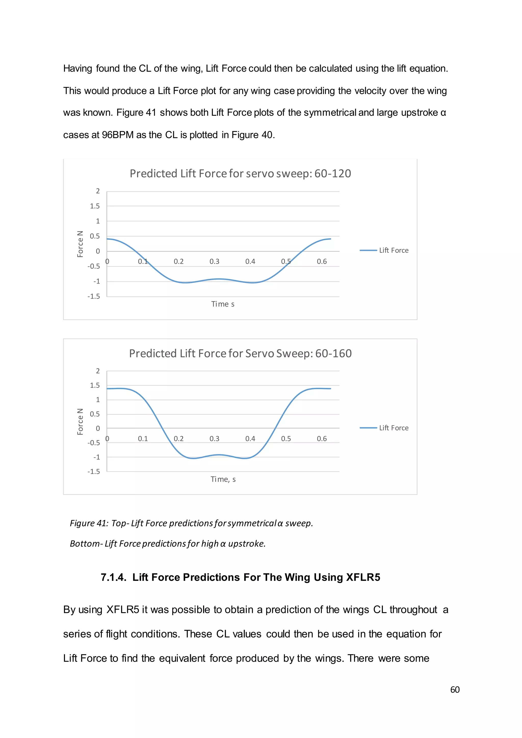
88. 88
find CL and then Lift Force which could be plotted alongside that obtained
experimentally for comparison. The Lift Force obtained from the load cell was
averaged over six wing beats in order to give an average set of values for a single
flap cycle. This approach to the theoretical calculations from the work of both
Whitney, J.P. (2012) [22] and Dickinson, M.H. (1999) [23] proved the most
straightforward way of processing the large amount of data generated in testing. This
coupled with the method of presenting experimental results by Sane, S.P. (2001) [2]
provided the best way of presenting both the predicted and actual values for a
specific combination of the frequency and amplitude of α applied to the test rig
wings.
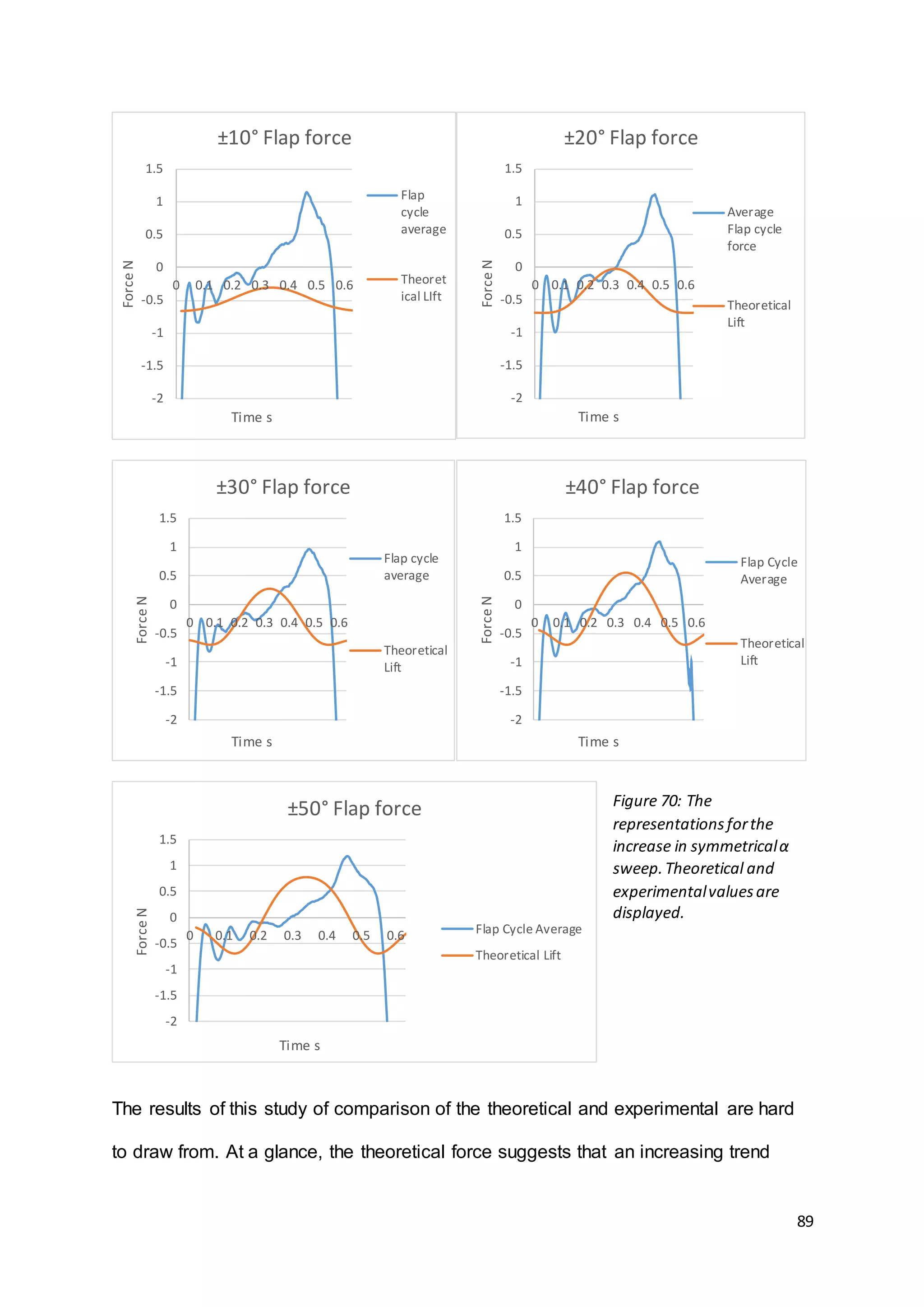
Figure 70 shows the plots of theoretical and experimental results for the testing of
increasing Angle of Attack. As much as possible, parameters were kept constant
across all testing with the same frequency, same conditions and the servos moving
the wings between positive and negative α at a uniform speed. Again as in previous
discussion over the theoretical results, the velocity applied in the equation for Lift
Force is not 0m/s which would be the true horizontal component of velocity on the
test rig wings. The freestream speed was again treated as 2m/s with the increase
induced by the wings flapping at 88 beats per minute. This allowed the aerodynamic
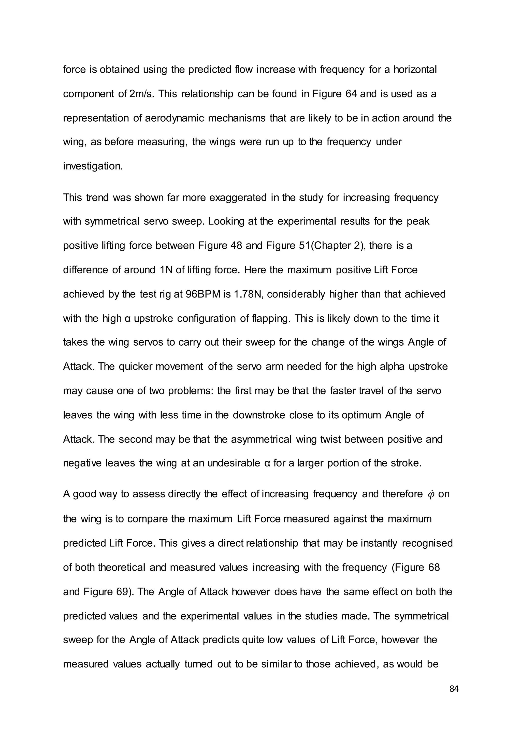
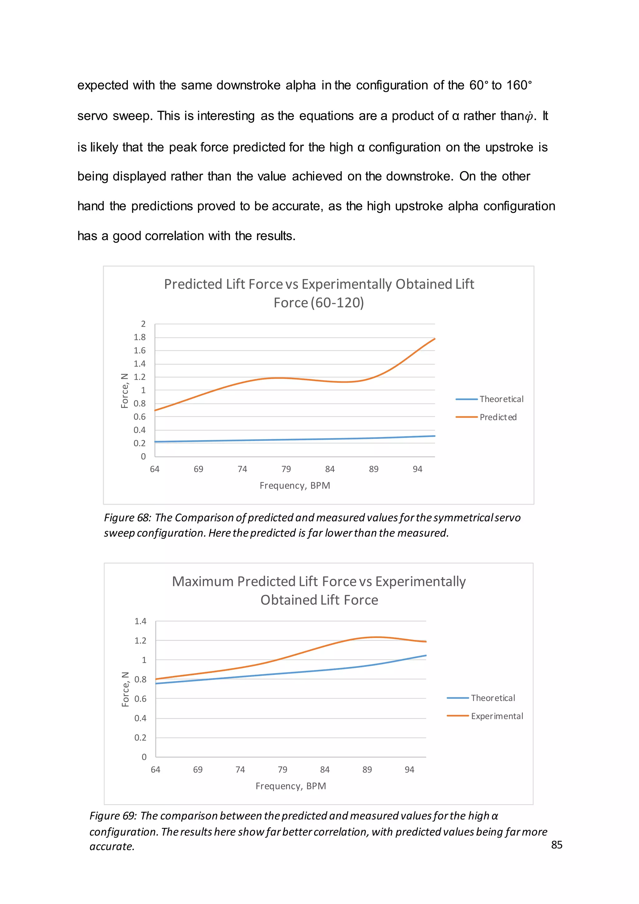
mechanisms and the motion of the wings to be accounted for in force calculations.

89. 89
The results of this study of comparison of the theoretical and experimental are hard
to draw from. At a glance, the theoretical force suggests that an increasing trend
-2
-1.5
-1
-0.5
0
0.5
1
1.5
0 0.1 0.2 0.3 0.4 0.5 0.6
ForceN
Time s
±10° Flap force
Flap
cycle
average
Theoret
ical LIft
-2
-1.5
-1
-0.5
0
0.5
1
1.5
0 0.1 0.2 0.3 0.4 0.5 0.6
ForceN
Time s
±20° Flap force
Average
Flap cycle
force
Theoretical
Lift
-2
-1.5
-1
-0.5
0
0.5
1
1.5
0 0.1 0.2 0.3 0.4 0.5 0.6
ForceN
Time s
±30° Flap force
Flap cycle
average
Theoretical
Lift
-2
-1.5
-1
-0.5
0
0.5
1
1.5
0 0.1 0.2 0.3 0.4 0.5 0.6
ForceN
Time s
±40° Flap force
Flap Cycle
Average
Theoretical
Lift
-2
-1.5
-1
-0.5
0
0.5
1
1.5
0 0.1 0.2 0.3 0.4 0.5 0.6
ForceN
Time s
±50° Flap force
Flap Cycle Average
Theoretical Lift
Figure 70: The
representationsforthe
increase in symmetricalα
sweep.Theoretical and
experimentalvaluesare
displayed.

90. 90
should be seen in the peak Lift Force achieved, however it seems to remain more or
less constant for all cases but 40° α, which drops as an anomaly. This result was
unexpected as it was assumed that an increasing value of Angle of Attack in the
downstroke would allow for better performance into the effective on coming flow and
provide better lifting capabilities.
The lack of a trend in the results could be the product of a number of factors. The
first possibility could be that in fact the 88 beats per minute was not high enough to
produce the force needed for a good analysis. As was found in the frequency study,
the increase in frequency would have induced an increase in forces measured.
Another factor could be the lack of oncoming flow over the wing. The incremental
changes in peak Lift Force predicted with increase in α do suggest that forces would
be as high as those found in the frequency study, with no prediction being 1N of
force or more. An oncoming flow of 2m/s may have produced better results. The final
factor, could be as previously mentioned; the lack of sensors or a feedback loop in
the control. As it is hard to judge the timing of the flapping and Angle of Attack, it
may be that a change in α was not correctly timed in any of the tests.
In order to directly compare the difference between the predicted and theoretical
forces it is useful to look at the peak forces achieved. Figure 71 shows the peak
forces plotted against the sweep angle for α. Here we can see that the experimental
results, although showing a slight increase, are fairly inconsistent with the lowest
value seen at 30°α. The predicted results on the other hand show the expected
upward trend.

91. 91
-0.4
-0.2
0
0.2
0.4
0.6
0.8
1
1.2
1.4
10 20 30 40 50
Force,N
Angle of Sweep, °
Peak Lift ForcePredicted vs Peak Lift ForceMeasured
Predicted Force
Measured Peak Force
Figure 71: The peakforcevaluesshow the extentof the discrepancy between the
experimentaland predicted results.Furtherworkwould seek to providea conclusive
study in this area.

92. 92
9. Conclusion
The results of this project bring forward a number of conclusions which may be
backed up by the data collected and the work undertaken. The theoretical study and
application of blade element theory to the flapping wings determines that flow must
increase with an increase in frequency. From this it follows that an increase in lift is
to be expected which is confirmed by both experimental studies into the variation of
frequency, with both Figures 68 and 69 (Chapter 3) showing an upward trend in Lift
force measured.
The second point worth mentioning is the difficulty in predicting the Lift that can be
generated by a set of flapping wings in ‘Zero’ Velocity conditions. Any calculation
made to predict lift force will not be entirely accurate for the conditions experienced,
to this end, the velocity of flow over the wings must to some extent be assumed by
the application of velocity induced by the flapping motion, determined by the use of
blade element theory. This difficulty led to the disparities seen in the theoretical and
experimental values for the angle of attack variation study, and the symmetrical α
sweep increase in frequency.
It is extremely obvious in the measurements from the load cell that the inertial forces
present during the motion of the wings is considerably higher in magnitude than the
forces under investigation. These forces could have the effect of obscuring some
results as they are clearly the dominant force at work within the test rig. In order to
conduct some more conclusive testing, these would have to be addressed.
As a result of the data collected in this study it is obvious that the main parameter
investigated essential to generating a suitable Lifting Force, was the flapping
frequency. The results show conclusive evidence that the lift force is increased per

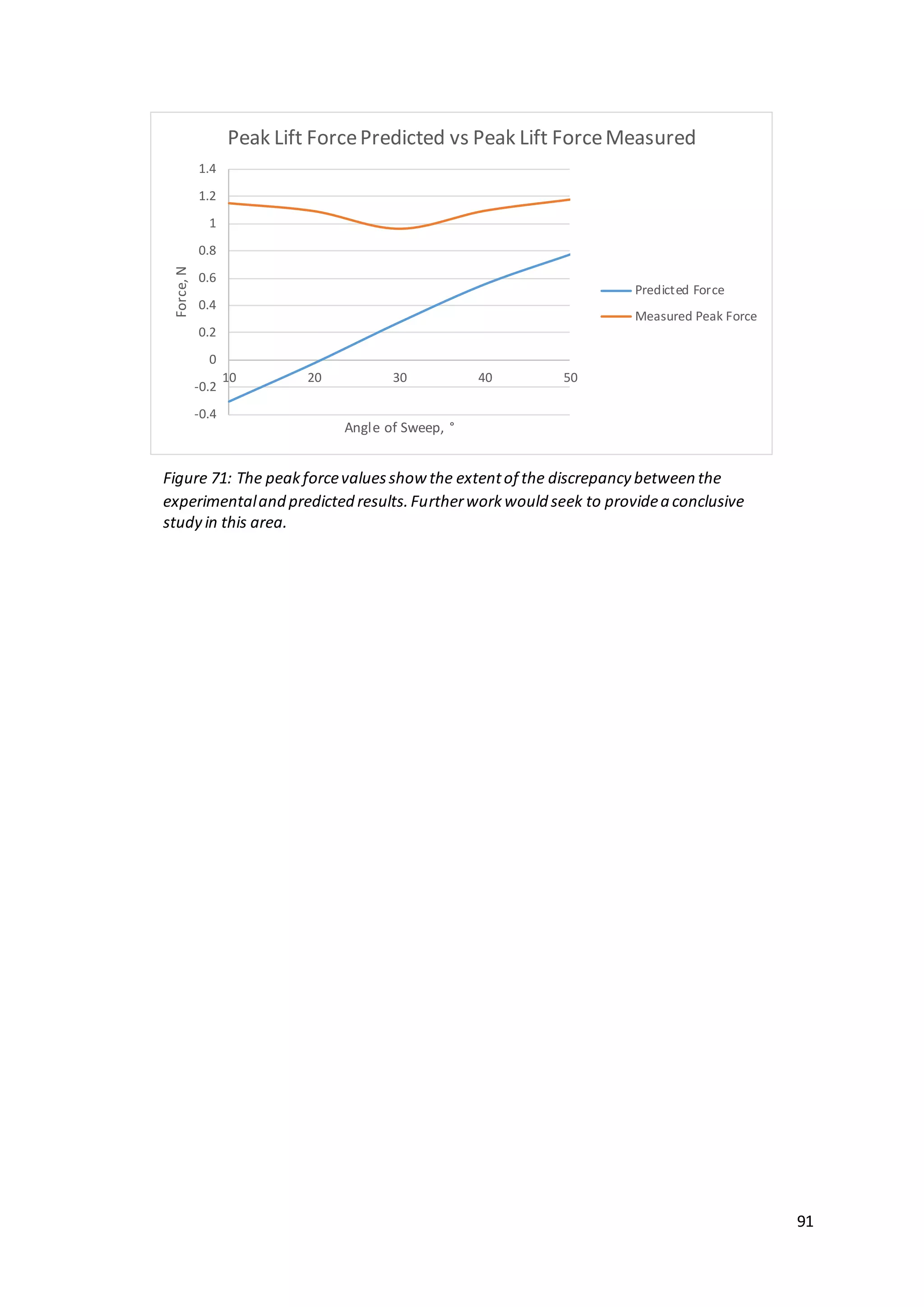
93. 93
stroke with higher frequency. It goes without saying that with higher frequency, the
force generated is applied more regularly per minute than the lesser force at a lower
amount of beats per minute. In the design of a flapping wing air vehicle, possibly the
most essential factor in its success would be to match the frequency with the
characteristics of the wings to ensure enough lift for the required performance. Angle
of Attack of the wings in the stroke, although important to some degree is thought
would be more essential in generating thrust which was not a subject of this project.
In further work there are many more alterations and measurements that would be of
use to the development of flapping wing flight. However as a result of this project and
specifically the work done in testing the concept of the flapping wings, with internal
servos providing wing twist, the main additional investigation would be as follows:
Firstly the investigations carried out in the results of this project, would be carried out
in some form of airflow, or the test rig attached to a rotating arm of constant speed.
This would allow forces to be measured outside of the zero velocity condition and
would allow the exact parameters used in the theoretical calculations to be
controlled. A second study to be carried out would be into the propulsive force
generated by the wings and the effect of the Angle of Attack and frequency on the
thrust the wings generate. For work such as this, it may also be of interest to add
some form of flexible trailing edge towards the tip of the wing, which could enhance
the thrust created significantly. Lastly the alteration off the design to the two panelled
wing configuration of the Festo Smartbird [3] would allow for a comparison of inertial
forces. The two panelled wing by its nature should provide a better conservation of
momentum in the flapping wings, due to the panels flapping out of phase. Forces at
the end of the down stroke would likely be far less in amplitude, with the entire flap
cycle being much smoother without the rapid change in direction of the wings seen

94. 94
with this apparatus. That is not to say however that with some design alterations, the
concept here could not be developed into a fully functioning MAV where the servos
used for wing twist could be used as a good substitute for the flexibility seen in
natural wings.

95. 95
10. References
1. Andrew M. Mountcastle, Stacey A. Combes (2013) 'Wing flexibility enhances load-
lifting capacity in bumblebees', Proceedings B, 280(1759), pp. 1-2 [Online]. Available
at:http://rspb.royalsocietypublishing.org/content/280/1759/20130531 (Accessed:
15/09/2015)
2. Sane, S.P.,Dickinson, M.H. (2001) 'The Control Of Flight Force By A Flapping Wing:
Lift And Drag Production', The Journal Of Experimental Biology, 204(JEB3400), pp.
2607-2626.
3. Festo (2011) Smartbird- Inspired by nature. [Online]. Available
at:http://www.festo.com/PDF_Flip/corp/smartbird_en/index.htm#/58/ (Accessed: 3rd
June 2015).
4. Festo (2013) BionicOpter - Inspired by Dragonfly Flight, Available
at:http://www.festo.com/net/SupportPortal/Files/248133/Festo_BionicOpter_en.pdf(A
ccessed: 3rd June 2015).
5. Festo (2015) eMotionButterflies - Ultralight flying objects with collective
behaviour,Available
at:http://www.festo.com/net/SupportPortal/Files/367913/Festo_eMotionButterflies_en.
pdf(Accessed: 3rd June 2015).
6. Lauri Poldre (2011) An interview with the engineer behind the man-made
SmartBird.,Available at: http://blog.grabcad.com/blog/2011/06/14/festo-
smartbird/ (Accessed: 4th June 2015).
7. Image Available from: http://www.festo.com/cms/en_corp/13165.htm
8. Nico Nijenhuis (2014) Clear Flight Solutions, Available
at:http://clearflightsolutions.com/ (Accessed: 4th June 2015).
9. Colin Jeffrey (2014) Robotic raptors look and fly like the real thing, Available
at:http://www.gizmag.com/flying-robot-raptor-birds-deter-nuisance-
flocks/33563/(Accessed: 4th June 2015).
10. Kyle Vanhemert (2014) Realistic Robo-Hawks Designed to Fly Around and Terrorize
Real Birds, Available at: http://www.wired.com/2014/08/realistic-robo-hawks-
designed-to-fly-around-and-terrorize-real-birds/ (Accessed: 4th June 2015).
11. Withers, P. C. An aerodynamic analysis of birds wings as fixed aerofoils. J. Exp.
Biol., 1981, 90, 143–162
12. Liu, T. , Kuykendoll, K. , Rhew, R., and Jones, S. Avian wing geometry and
kinematics. AIAA J., 2006, 44, 954–963.
13. BROWN, R.E., FEDDE, M.R. (1993) 'Airflow Sensors in the avian wing', Journal of
Experimental Biology, 179(66506), pp. 13-30.
14. Carruthers A.C.∗, Walker S.M., Thomas A.L.R., Taylor G.K. (2009) 'Aerodynamics of
aerofoil sections measured on a free-flying bird', Part G: J. Aerospace
Engineering,224(AERO737), pp. 855-864.
15. Bilo, D. Flugbiophysik von Kleinvögeln. I. Kinematik und Aerodynamik des
Flügelabschlages beim Haussperling (Passer domesticus L.). Z. vergl. Physiol.,
1971, 71, 382–454
16. Brill, C., Mayer-Kunz, D. P., and Nachtigall,W.Wing pro- file data of a free-gliding
bird. Naturwissenschaften, 1989, 76, 39–40.
17. Heather Howard (2014) Falconsong Studios, Available
at:http://www.falconsongstudios.com/?page_id=844 (Accessed: 9th June 2015).
18. Andrew A. Biewener (2011) 'Muscle function in avian flight: achieving power and
control', Integration of muscle function for producing and controlling
movement,366(1570), pp. 3-15 [Online]. Available
at:http://rstb.royalsocietypublishing.org/content/366/1570/1496 (Accessed: 9th June
2015).
19. Image available from: http://www.birdsnways.com/wisdom/ww19eii.htm

96. 96
20. Micheal L. Anderson, Major, USAF, “Design and Control of Flapping wing
MAV’s”,Department of Airforce Air university, Airforce institute of technology, Wright-
Patterson AFB, Ohio (2011).
21. Le, M. (2012) An Unconventional Lift-Enhancing Mechanism: Clap and
Fling, Available at: http://blogs.bu.edu/bioaerial2012/2012/12/08/an-unconventional-
lift-enhancing-mechanism-clap-and-fling/ (Accessed: 11th June 2015).
22. Whitney, J.P., 2012. Conceptual design of flapping-wing micro air vehicles. Doctoral.
Cambridge, MA 02138: Harvard University.
23. Dickinson, M.H., Lehmann, F.O., Sane, S.P. (1999) 'Wing Rotation and the
Aerodynamic Basis of Insect Flight', Science, 284(5422), pp. 1954-1960.
24. Zhao, L, Huang, Q, Deng, X, Sane, S.P (2010) 'Aerodynamic effects of flexibility in
flapping wings', The Royal Society of Publishing 'Interface', 7(44)
25. Images availiable at: http://m-selig.ae.illinois.edu/ads/coord_database.html
26. Image availiable at: http://www.wfis.uni.lodz.pl/edu/Proposal.htm
27. Robert S. Merrill (2011) Nonlinear Aerodynamic Corrections to Blade Element
Momentum Modul with Validation Experiments, Logan, Utah : Utah State University,
(p5-p11)
28. D.J. Auld, K. Srinivas (1995-2006) Aerodynamics for Students - Blade element
propeller analysis, Available at: http://www-
mdp.eng.cam.ac.uk/web/library/enginfo/aerothermal_dvd_only/aero/propeller/prop1.h
tml(Accessed: 8th July 2015).

97. 97
11. Project Management
Shown in Figure 1 is the original plan proposed for the project, however this was
subject to some change in the duration of the project for various reasons. The first
difference one can notice in the actual timescale shown in Figure 2, Is the changes
in some of the tasks to be carried out. The main differences occur at the bottom of
the task list where original work proposed was slightly over ambitious with not
enough time being left to test the propulsive force of the test rig. This would have
required considerably more time with a considerable amount of change needed in
order to change the plane of the load cell by 90°, and not to mention a new way of
supporting the frame.
Figure 1: The Original GanttChartplan forthe project

98. 98
Figure 2 has another difference in that the experimental work is pushed much further
towards the end of the project. This came as a result of an unexpected amount of
time needed to order and obtain specific parts for the project, such as the load cell
and the hinges. This situation of parts not being always available at the planned time
pushed back the construction of the wings and mechanism and delayed the test rig
calibration and set-up. Had these unexpected circumstances not been present
however, it is likely the last part of the project would have run much closer to
schedule.
Figure 2: This showstheactual timingsof the projectand the changesin the stepsto be taken
are included with minorchangesmadeto the tasklist.

99. 99
12. Appendix: Dissertation Proposal: Bio-inspired
Flying Machines
1. Introduction and Background to the Project
There is currently a fast increasing interest in bird and insect flight and how this
could be interpreted into a mechanical flying machine, more specifically in the form
of a UAV (unmanned air vehicle). Potential for such vehicles has been identified in a
number of sectors, most notably in the military market. With development of stealth
technology and radar being in a constant battle of development, a new form of
stealth is being considered, in the form of ‘bird or insect like’ vehicles. These would
be small and disguised to look as their counterparts in the natural world making them
very hard to detect visually and by radar. Lessons have already been learn for the
current generation of small UAV’s as birds and insects have naturally evolved to
operate in similar Reynolds number regimes [1].
Many attempts have been made to achieve flapping wing flight as it has been a
dream of man-kind for century’s to fly like a bird resulting in many ornithopter
attempts and to this day models are still being produced for hobbyists, some
powered by elastic bands, others powered by electric motors. However perhaps
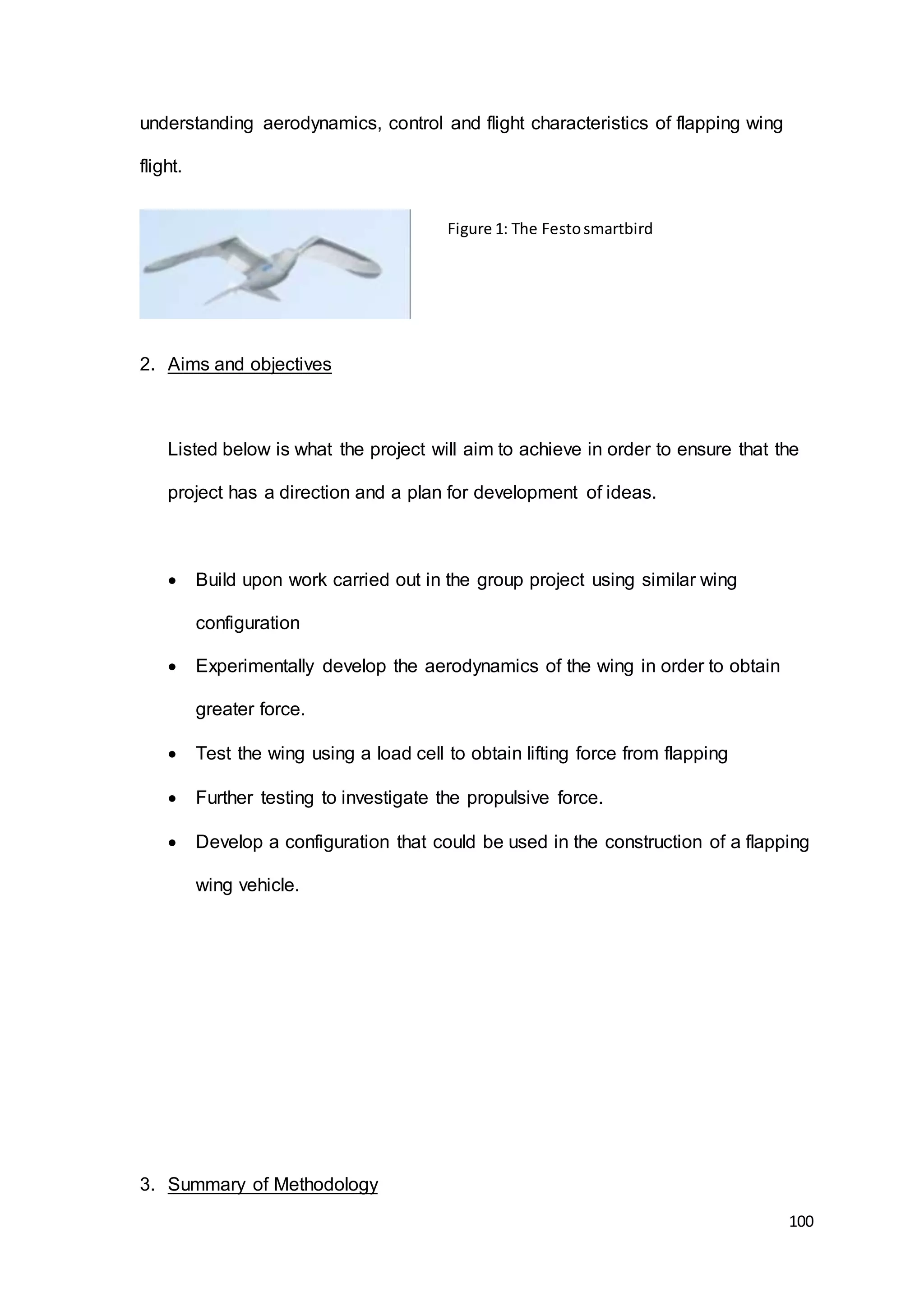
the most significant step forward in bird like flight is the FESTO Smartbird, based
on a gull (Figure 1). This uses flapping with a servo to actively twist the wing
based on sensor readings for torsion of the wing, load on the motor and motor
position. Other vehicles have also been produced drawing inspiration from other
areas such as hummingbirds, dragonflies and other insects, however most of
these are much smaller and the end result is not as convincingly real.
Nonetheless, some of these have also provided major leaps forward in

100. 100
understanding aerodynamics, control and flight characteristics of flapping wing
flight.
2. Aims and objectives
Listed below is what the project will aim to achieve in order to ensure that the
project has a direction and a plan for development of ideas.
 Build upon work carried out in the group project using similar wing
configuration
 Experimentally develop the aerodynamics of the wing in order to obtain
greater force.
 Test the wing using a load cell to obtain lifting force from flapping
 Further testing to investigate the propulsive force.
 Develop a configuration that could be used in the construction of a flapping
wing vehicle.
3. Summary of Methodology
Figure 1: The Festosmartbird

101. 101
 Review literature and summarise the findings with a specific focus on wing
profiles, shapes. Look also at models and equations for lift generated by
wing flapping relating to angle of attack to the oncoming flow
 Learn how to program an Arduino board, this will be useful when it comes
to testing as the correct motors and servos will be able to set up in order to
control the test and gain accurate results.
 Produce CAD models of wing designs for both preliminary analysis and for
ease of producing accurate components in experimental testing.
 Design and build prototype wings and test rig. It is essential that the
different test subjects may be interchanged easily without lengthy
adaptions or having to largely disassemble the experimental set-up.
 Produce a programmed electronic system using the Arduino set to be
applied to flap and twist the wings whilst being experimented on.
 Run a series of tests using a load cell mounted with the motors for the
electronic flapping in order to determine differences between test subjects.
 Test for propulsive force obtained from the wing using a similar load cell
configuration in the horizontal axis, rather than vertical.
 Attempt to apply results to build a full model for the configuration of a
flapping wing vehicle, this would follow work done in the group project
using a similar concept.
4. Project Plan

102. 102
References
1. Carruthers A.C.∗, Walker S.M., Thomas A.L.R., Taylor G.K. (2009) 'Aerodynamics of
aerofoil sections measured on a free-flying bird', Part G: J. Aerospace
Engineering,224(AERO737), pp. 855-864.

103. 103
13. Appendix
1- The outline of the frames for Laser Cutting
2-The File of the wing ribs to be laser cut.

104. 104
3. The Arduino Code
#include <Servo.h>
Servo escmot;
Servo myservo1;
Servo myservo2;
int pos = 0;
void setup() {
myservo1.attach(10);
myservo2.attach(11);
myservo1.write(100);
myservo2.write(90);
escmot.attach(9);
escmot.write(0);
delay(5000);
escmot.write(19);
delay(5000);
escmot.write(30);
delay(5000)
}
void loop() {
escmot.write(43);
for(pos = 70; pos < 170; pos +=3.5)
{
myservo1.write(pos);
myservo2.write(60+160-pos);
delay(15);}
for(pos = 160; pos>=60; pos-=3.2)
{
myservo1.write(pos);
myservo2.write(70+170-pos);
delay(15);}
}

105. 105
4. Picturesof the completedWingStructure

106. 106
5. Picture of the Test Rig and Experimental
Set-up