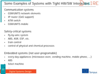
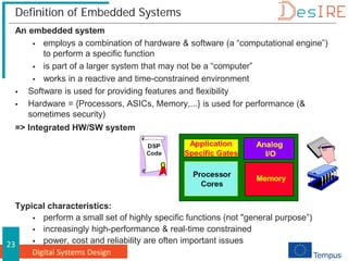
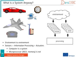
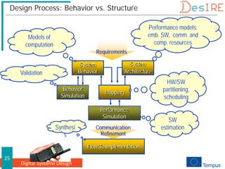
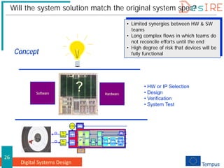
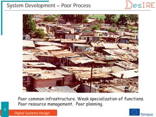
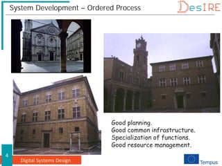
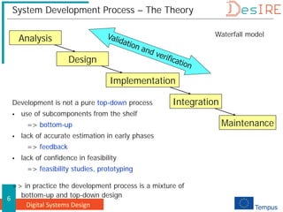
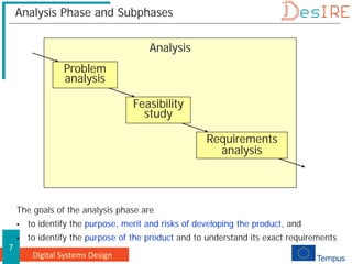
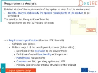
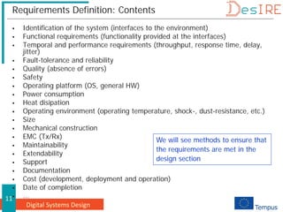
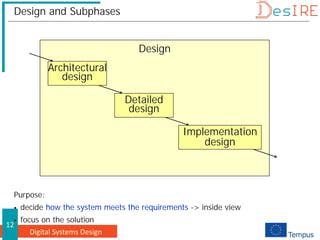
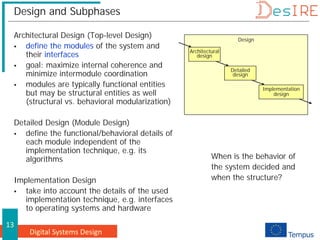
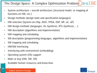
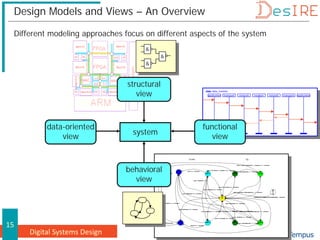
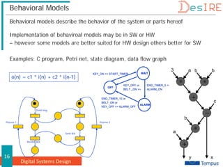
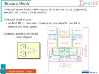
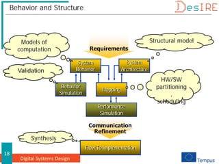
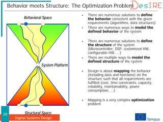
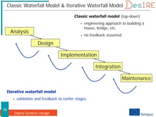
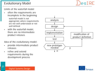
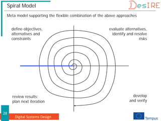
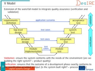
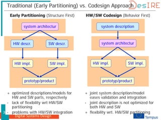
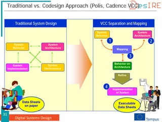
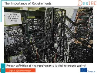
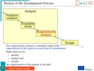
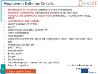
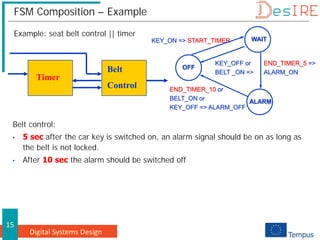
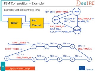
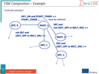
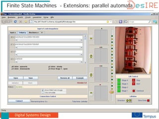
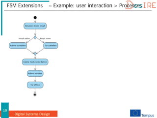
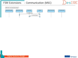
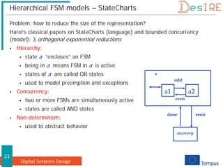
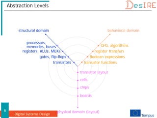
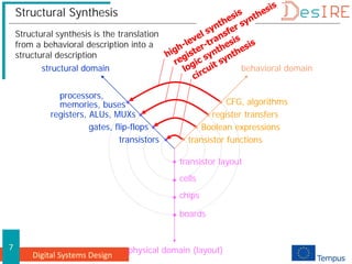
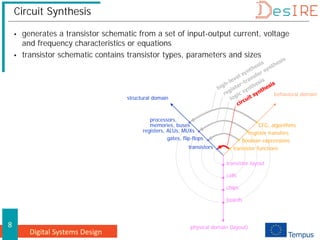
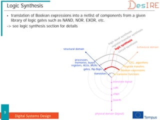
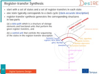
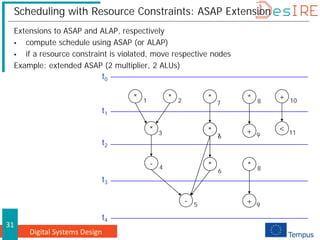
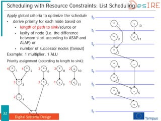
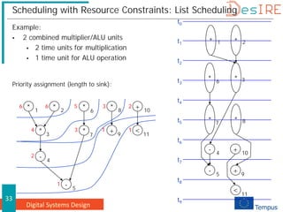
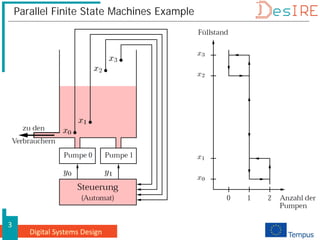
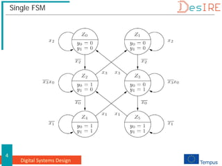
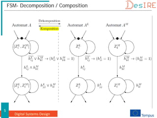
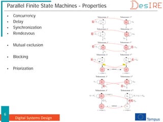
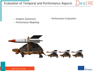
The document outlines a course on integrated hardware and software systems, emphasizing the importance of understanding hardware-software interaction for effective system design. It covers various systems requiring such integration, like embedded and safety-critical systems, and details the development process, including analysis, design, and implementation phases. The course aims to equip participants with the knowledge necessary to make informed design decisions across different applications and industries.


![Digital Systems Design
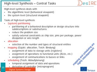
18
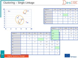
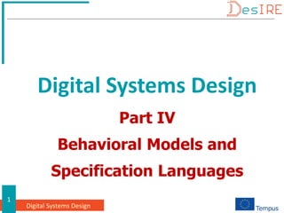
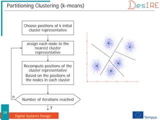
Clustering – Single Linkage
0
1
2
3
4
5
6
7
8
9
10
0 2 4 6 8 10
P1
P2
P3
P4
P5
P6
P7 Distance between groups is estimated as
the smallest distance between entities
Example:
[ ] 1
.
4
,
min 45
45
25
5
)
4
,
2
( =
=
= d
d
d
d
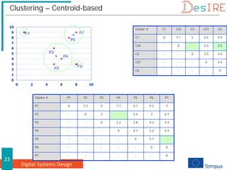
Cluster # P1 P2 P3 P4 P5 P6 P7
P1 0 7.2 5 7.1 6.1 9.2 7
P2 - 0 3 1.4 5.4 3 6.7
P3 - - 0 2.2 2.8 4.3 4.3
P4 - - - 0 4.1 2.2 5.4
P5 - - - - 0 5.1 1.4
P6 - - - - - 0 6
P7 - - - - - - 0](https://image.slidesharecdn.com/digitalsystemsdesign-241113201401-049b1be5/85/Digital-Systems-Design-description-and-implementation-pdf-254-320.jpg)