Download to read offline


![M. Junaid Mughal 2006
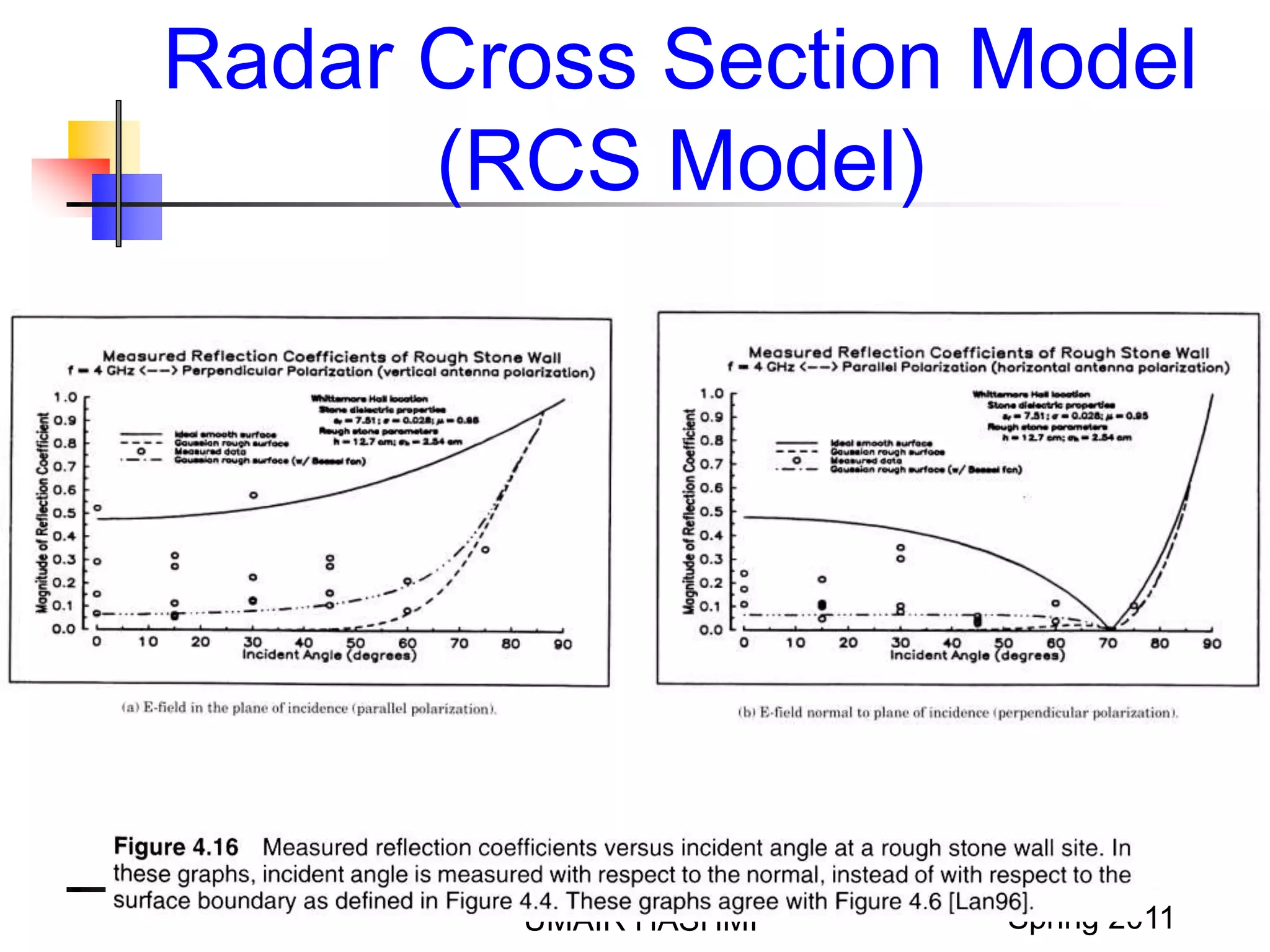
Radar Cross Section Model
(RCS Model)
UMAIR HASHMI Spring 2011
• The Radar Cross Section (RCS) of a scattering object is
defined as the ratio of the power density of the signal scattered
in the direction of the receiver to the power density of the radio
wave incident upon the scattering object.
• The bistatic radar equation is used to compute the
propagation of a wave travelling in free space that impinges on
a distant scattering object and then reradiated in the direction
of the receiver. The objects are assumed to be in the Far-Field
region (Fraunhofer region)
PR (dBm) = PT (dBm) + GT (dBi) + 20 log λ + RCS [dB m2 ] – 30
log (4 pi) – 20 log dT – 20 log dR](https://image.slidesharecdn.com/digitalclass-200131042600/75/Digital-class-31-2048.jpg)


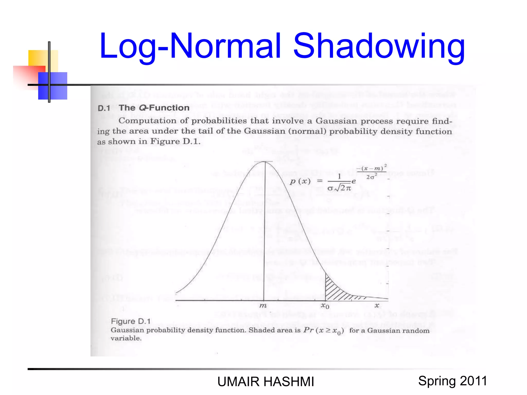


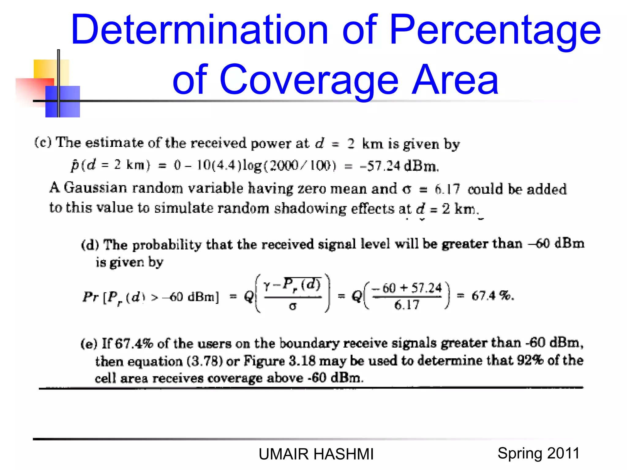


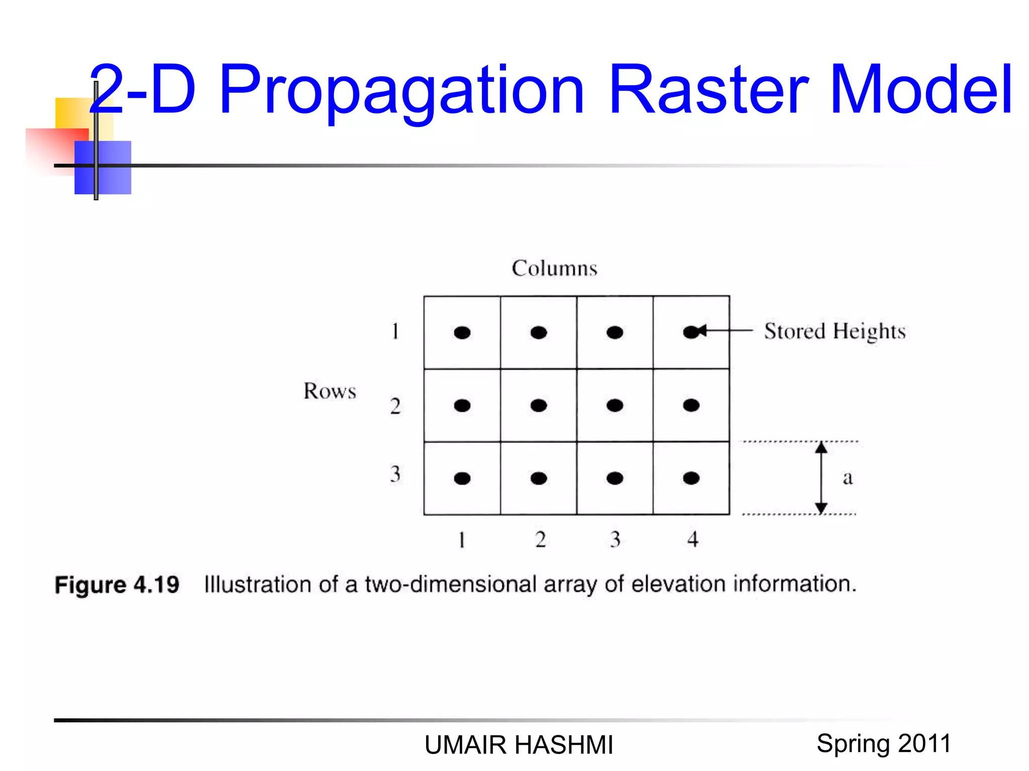
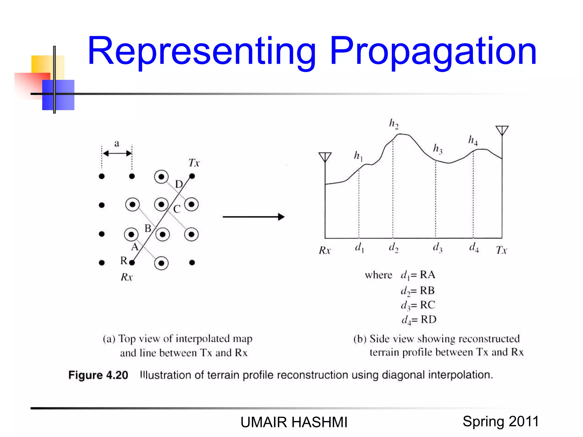
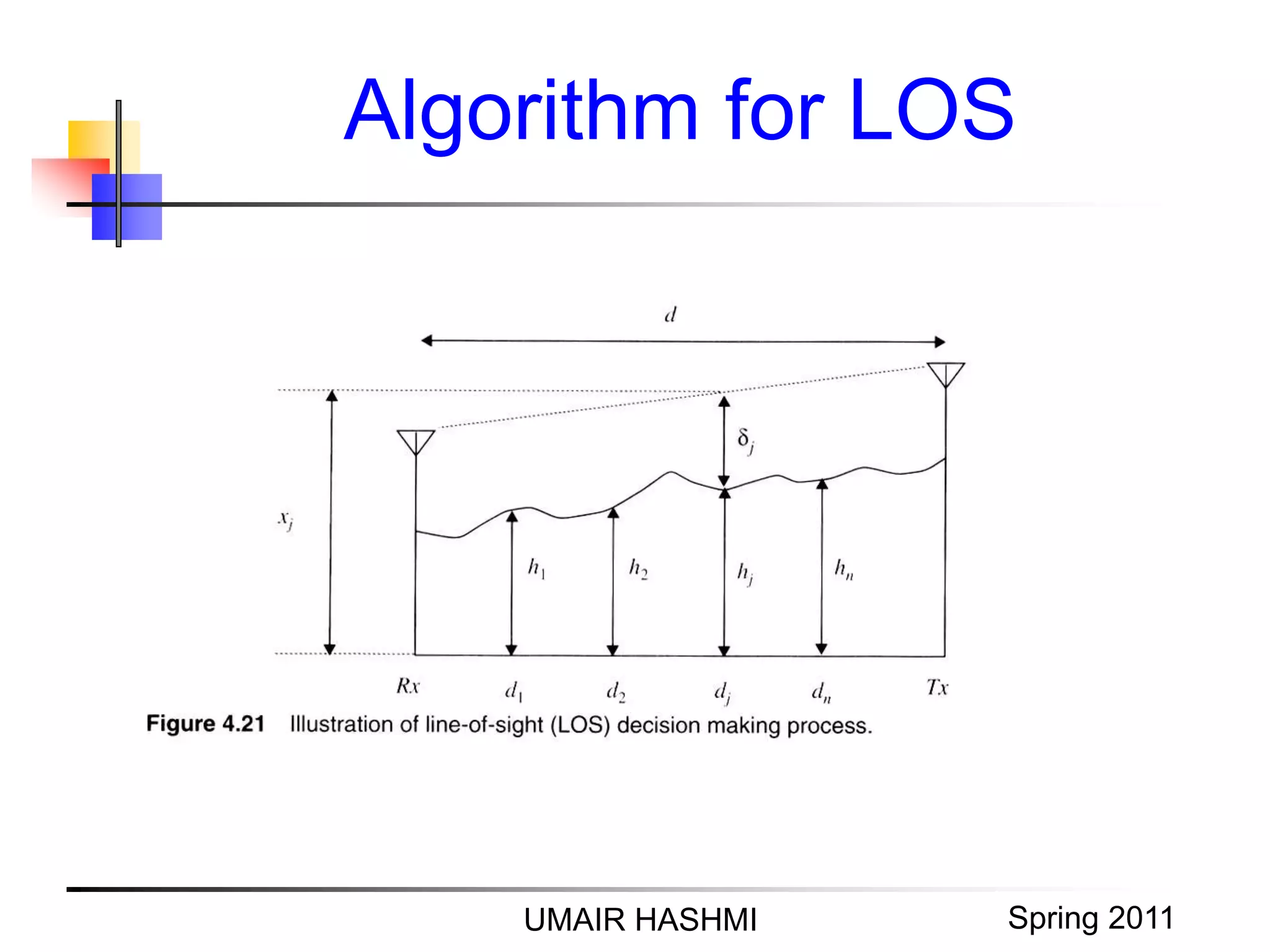


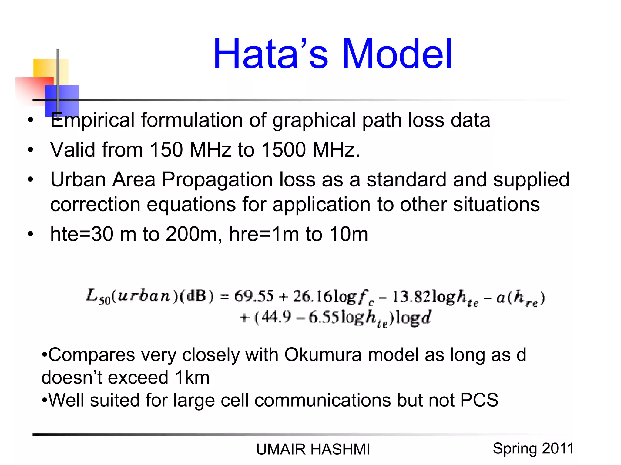


The document discusses several topics related to wireless propagation modeling including: 1. The log-distance path loss model, which models received power as decreasing logarithmically with distance. 2. Log-normal shadowing, which describes how multipath effects cause random variations in the received signal at a given distance. 3. Methods for determining the percentage of coverage area where the received signal is above a threshold, including calculating the complementary cumulative distribution function. 4. Outdoor propagation models including the Longley-Rice model, Durkin's model, and the two-ray propagation raster model for irregular terrain. 5. Empirical models like Hata's model and its extension to personal communication services frequencies


![Vibe Coding vs. Spec-Driven Development [Free Meetup]](https://cdn.slidesharecdn.com/ss_thumbnails/vibecodingvsspecdrivendevelopment-251209105622-43f455e7-thumbnail.jpg?width=640&height=640&fit=bounds)


