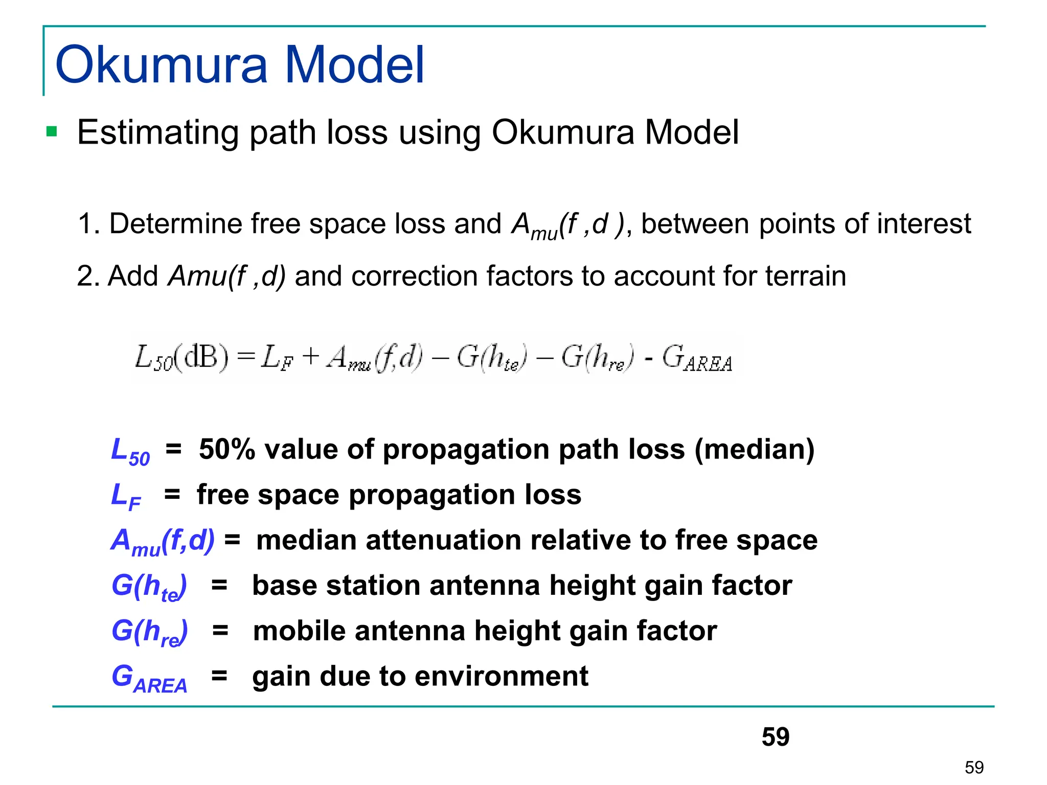
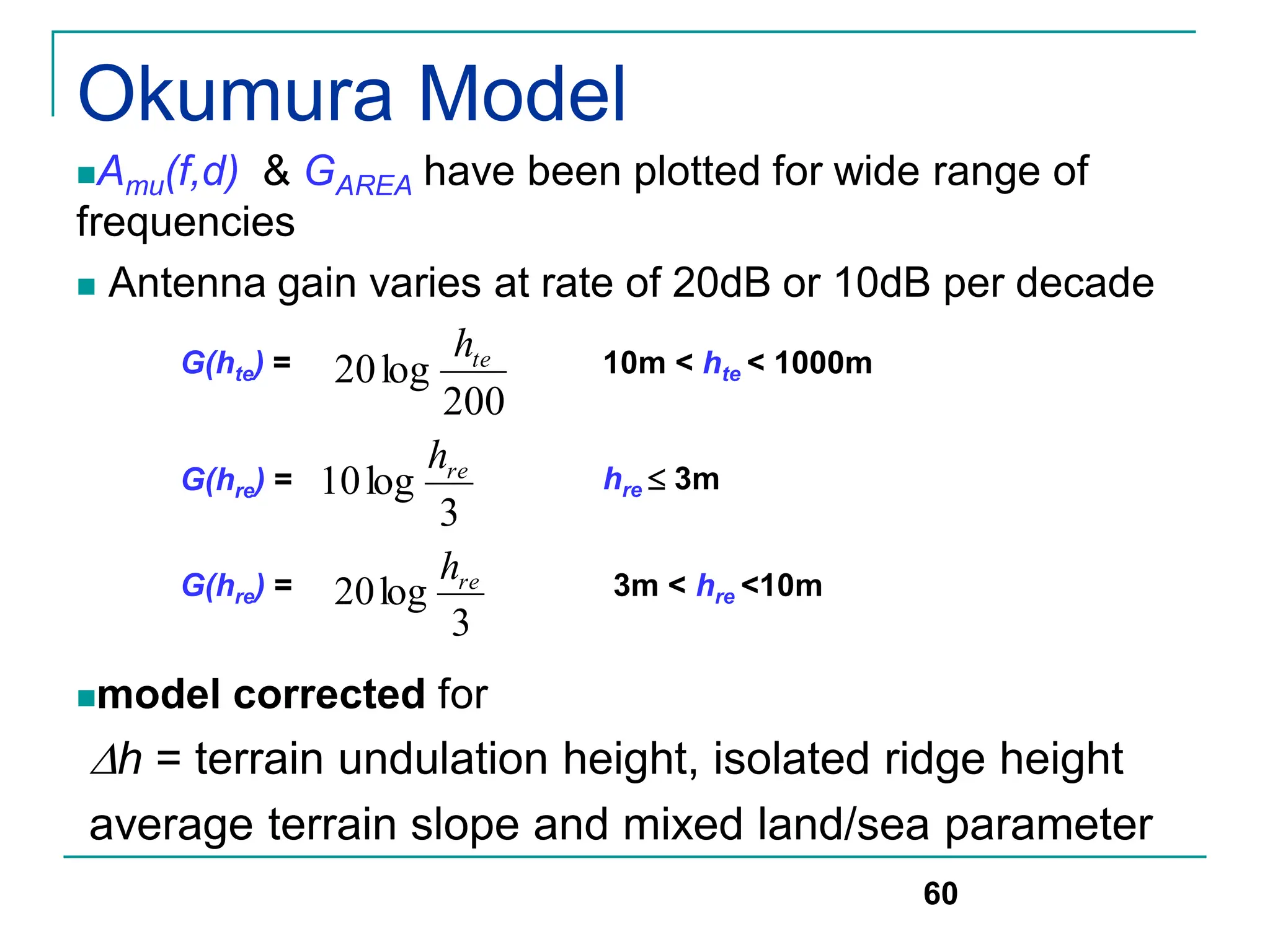
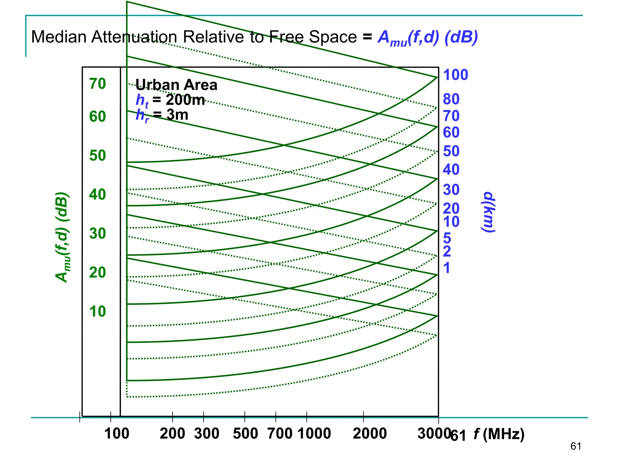
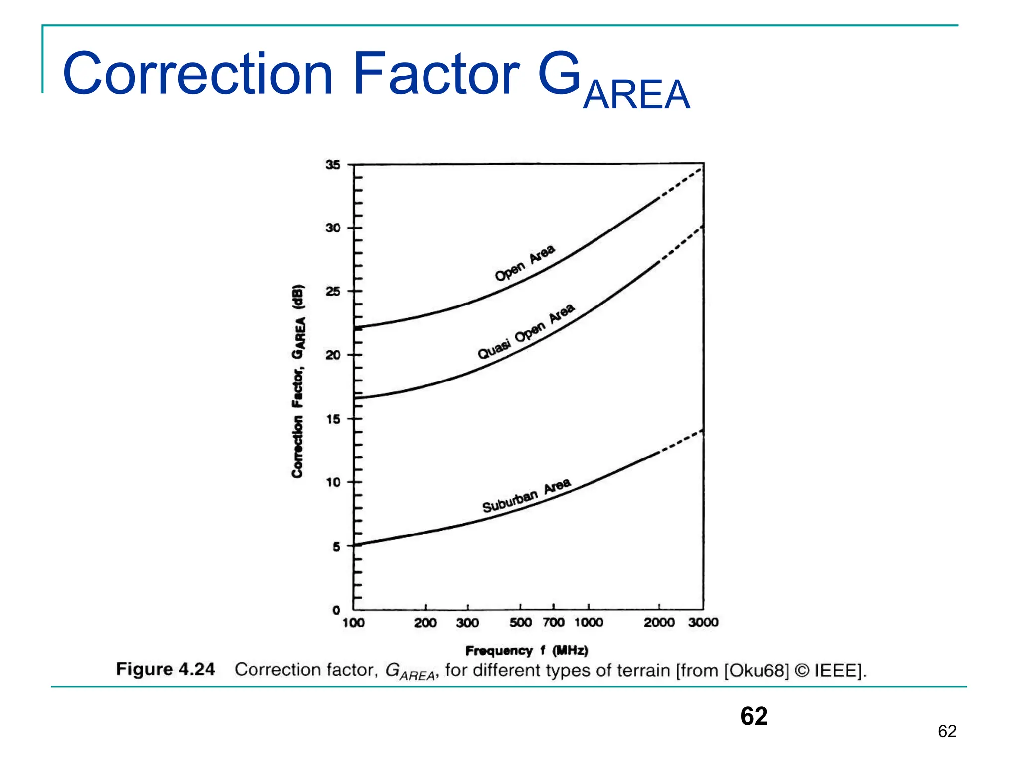
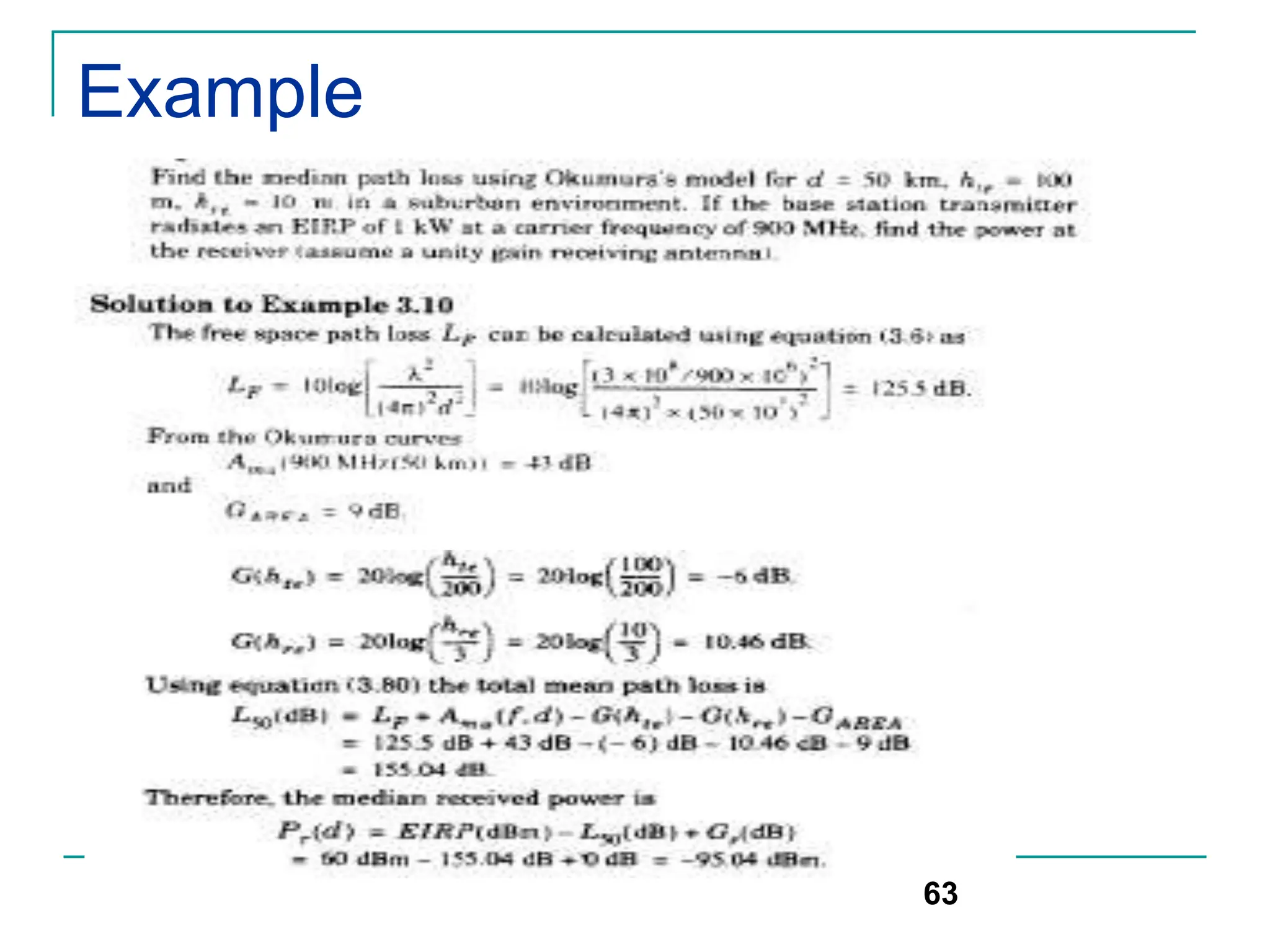
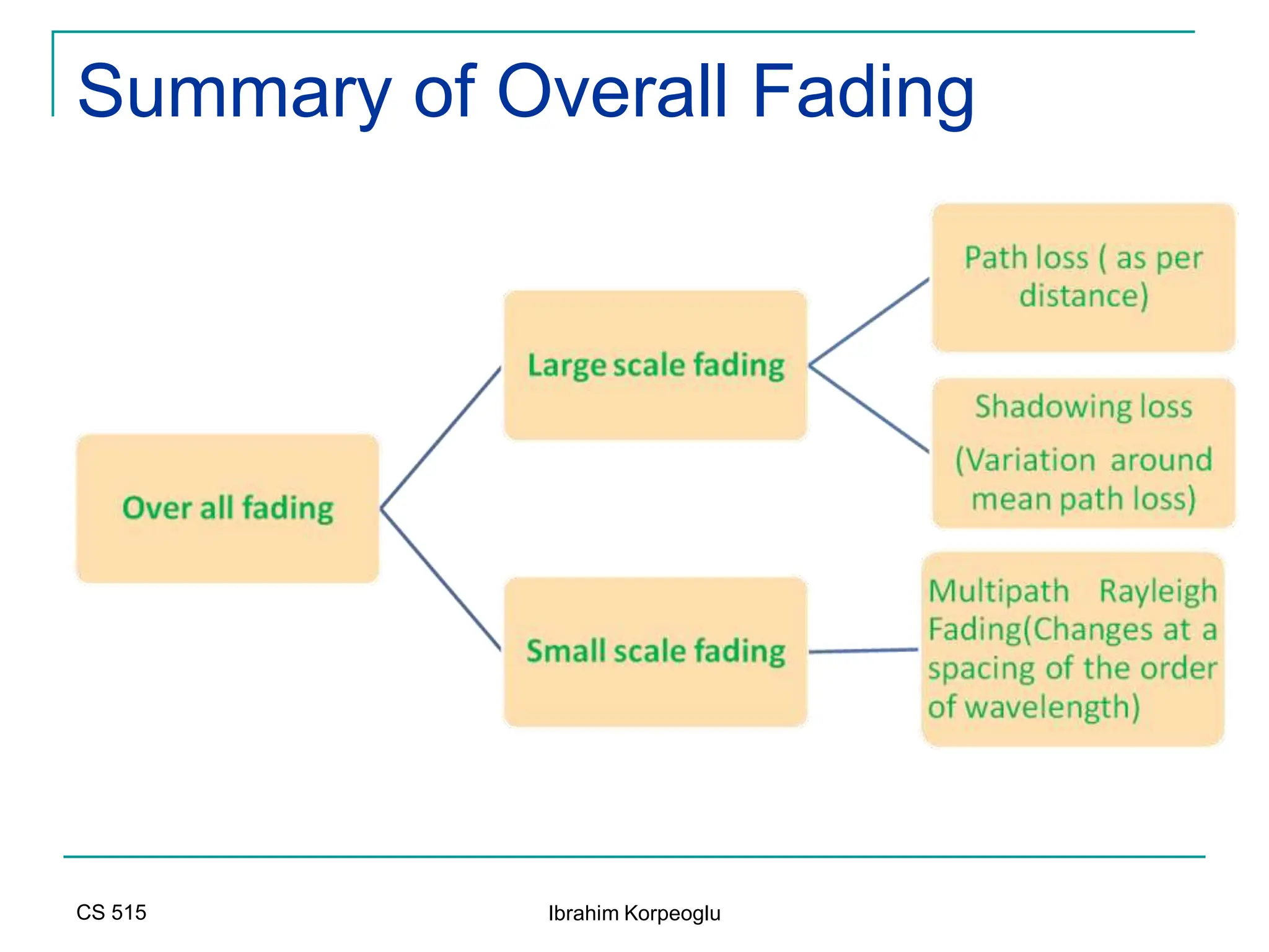
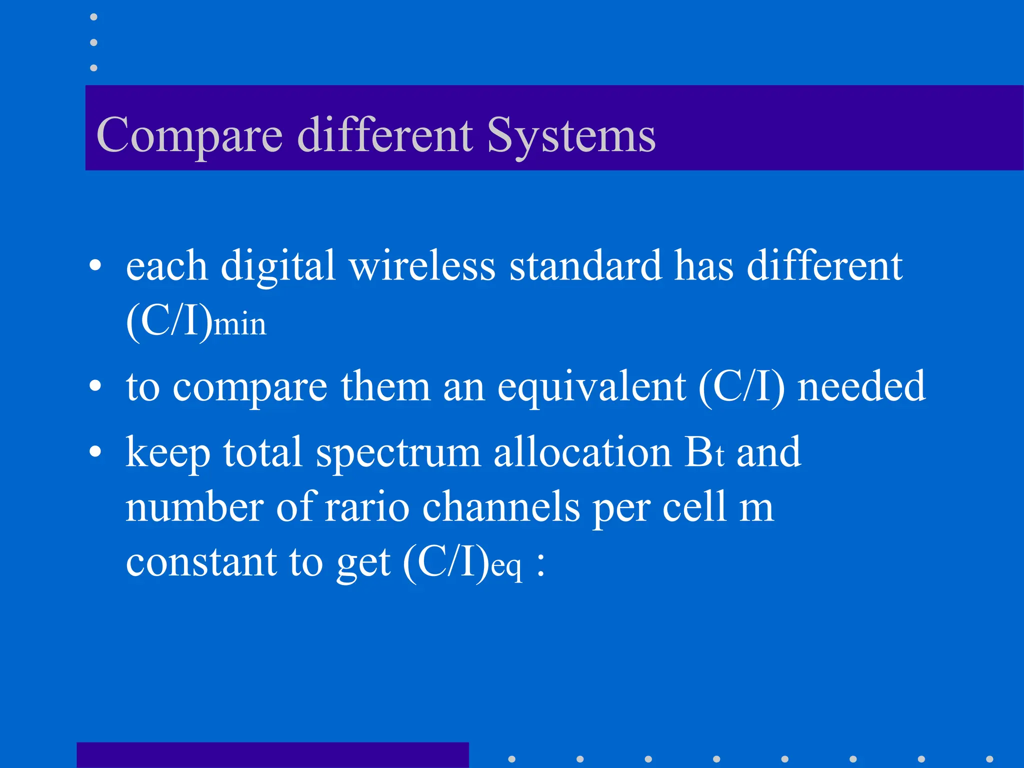
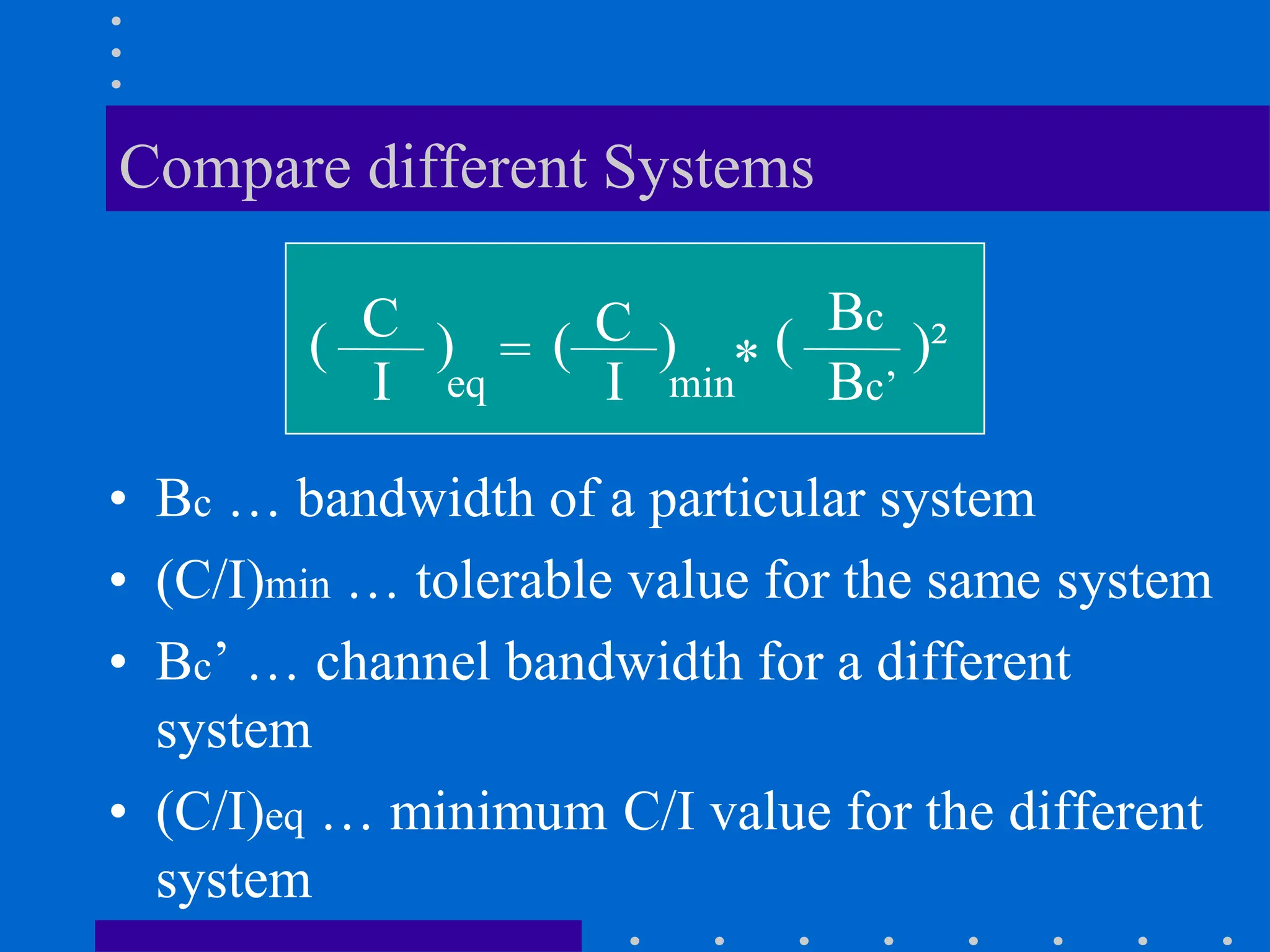
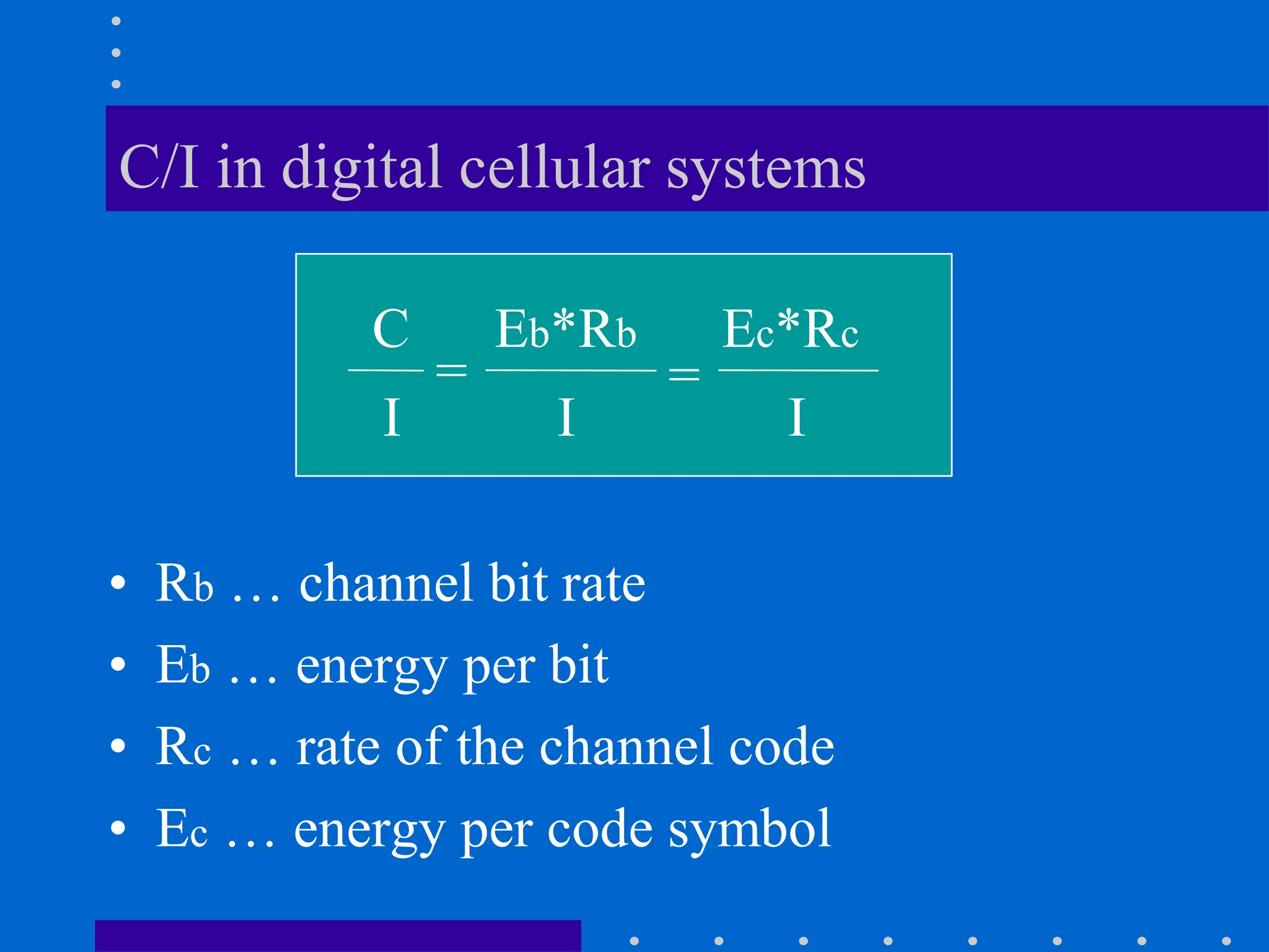
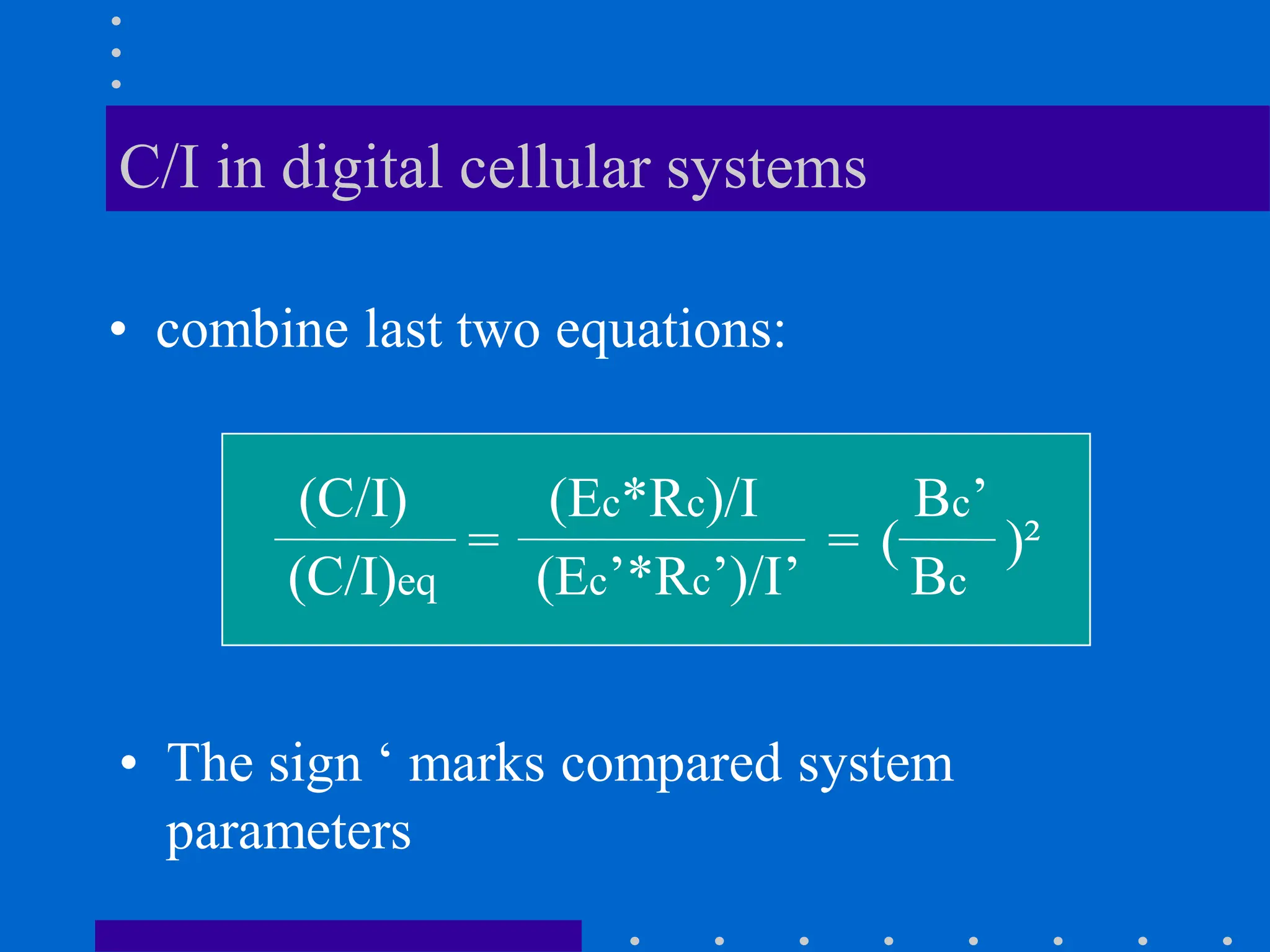
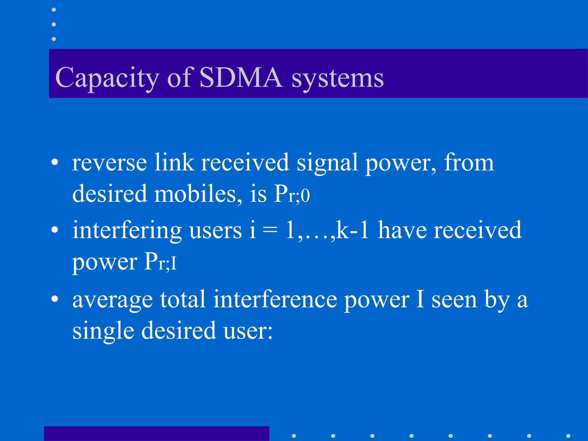
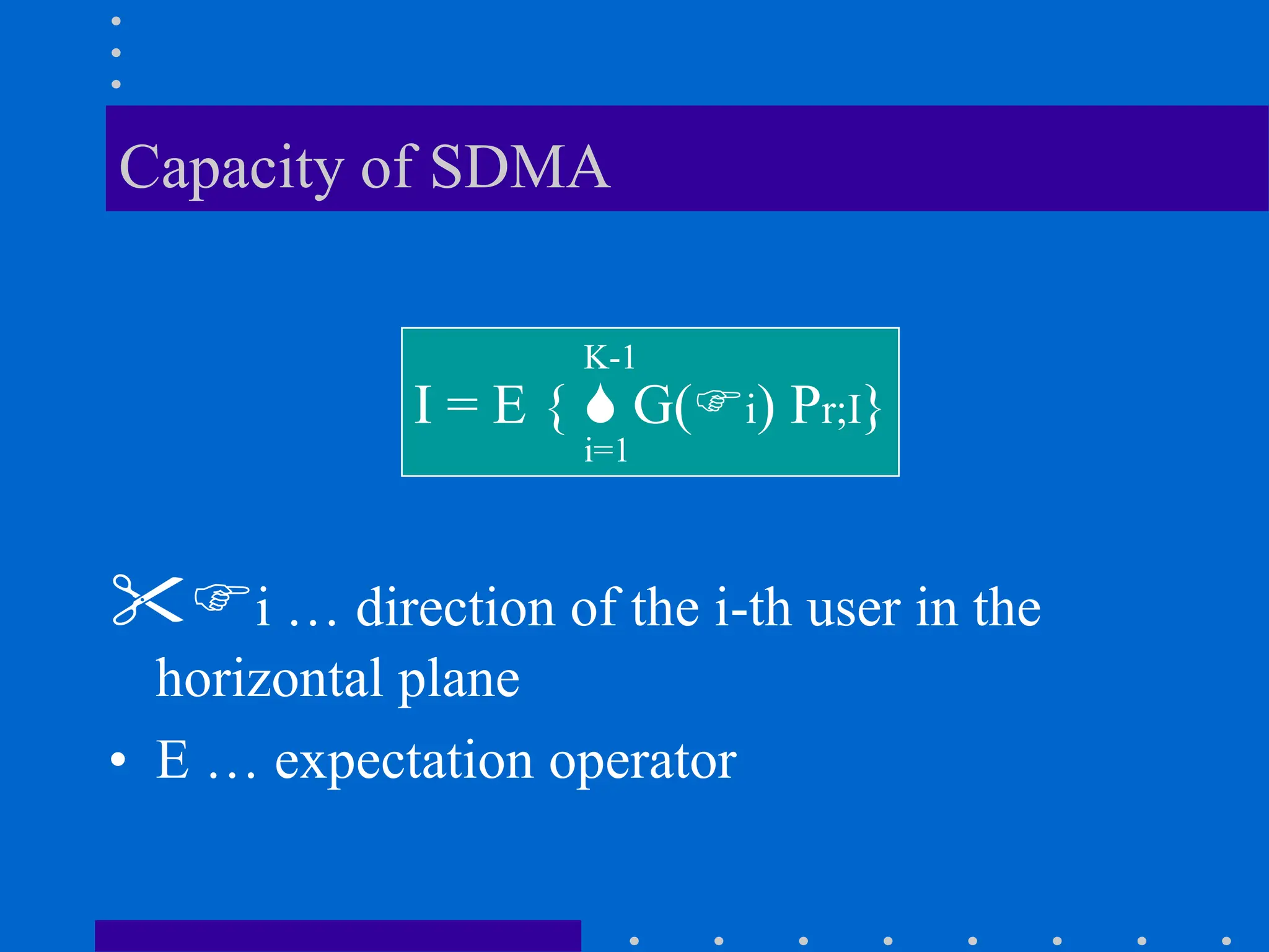
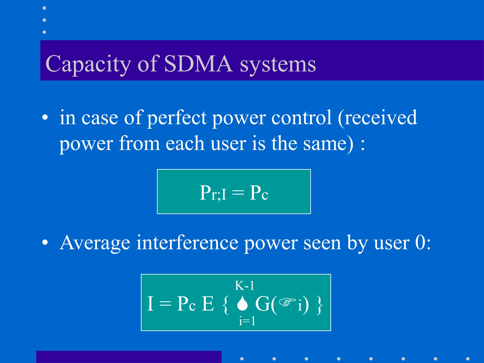
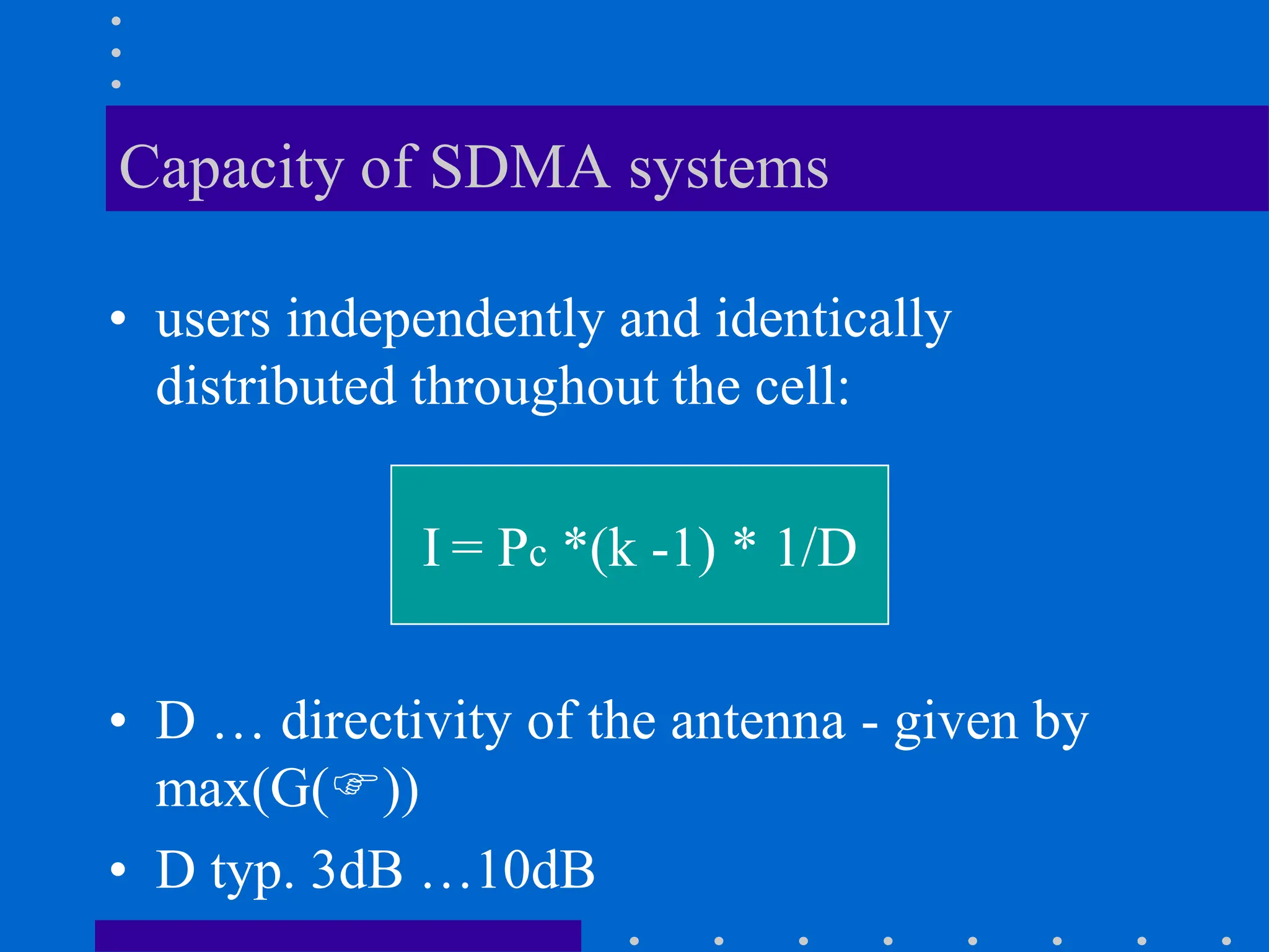
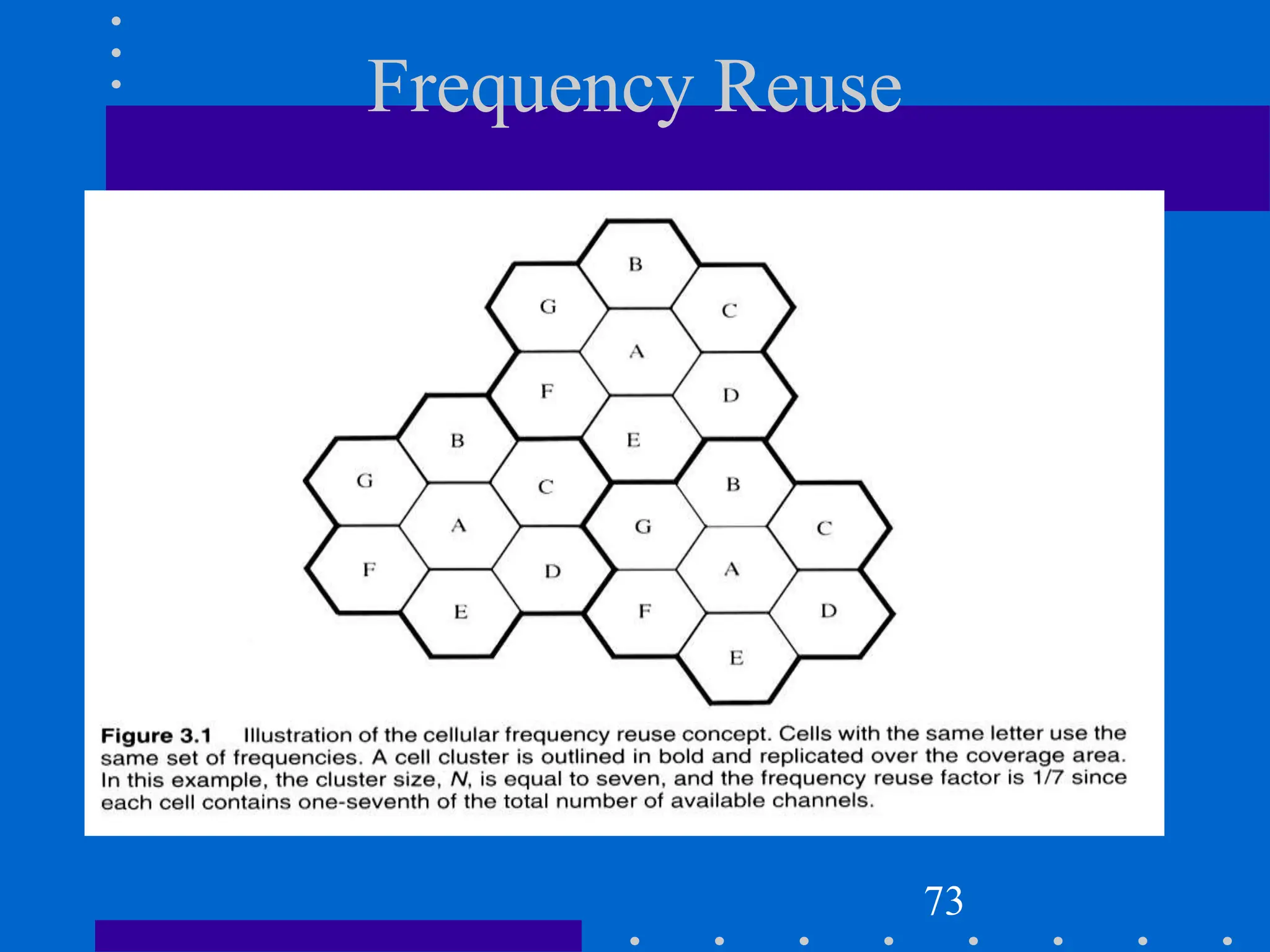
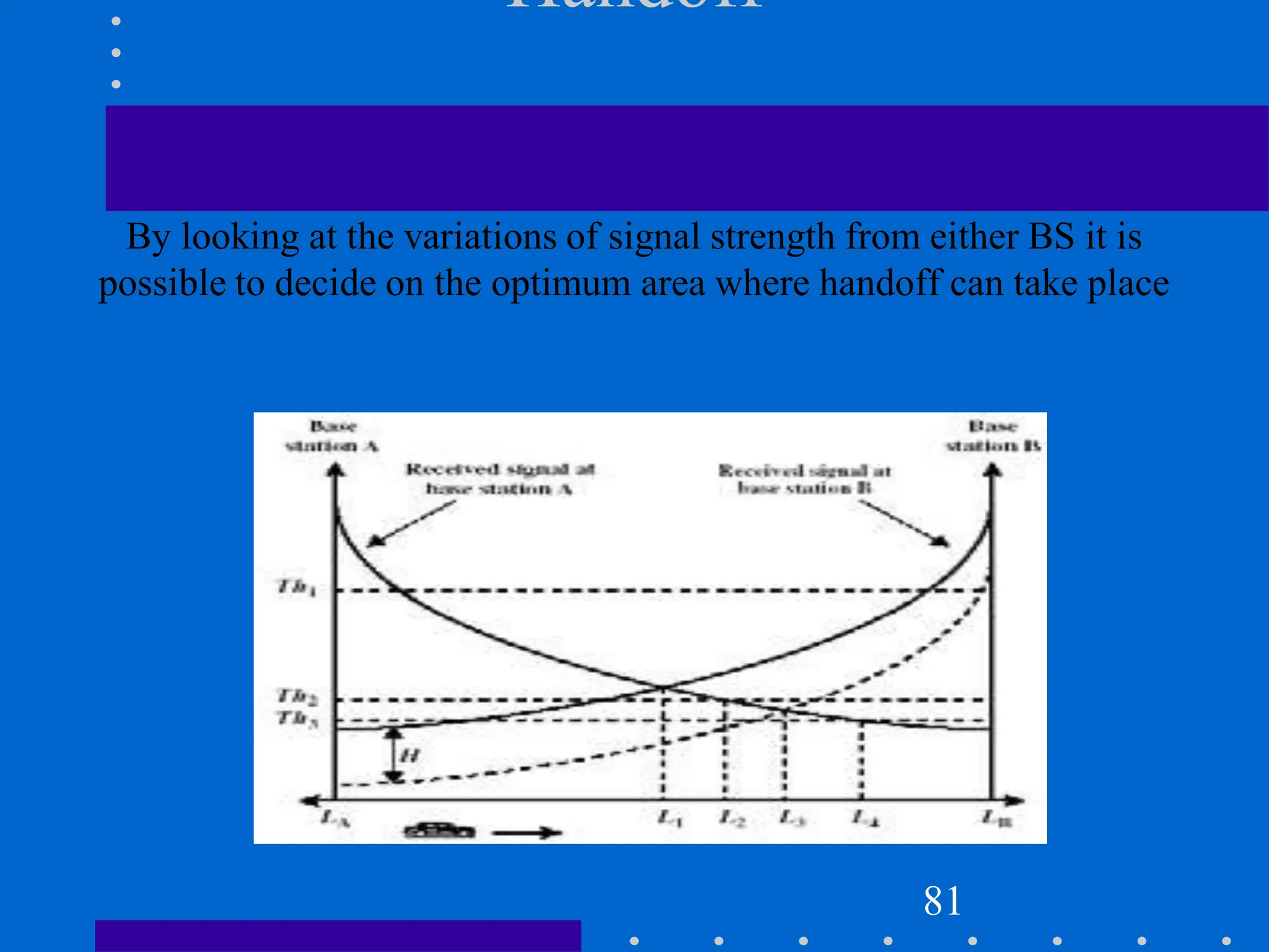
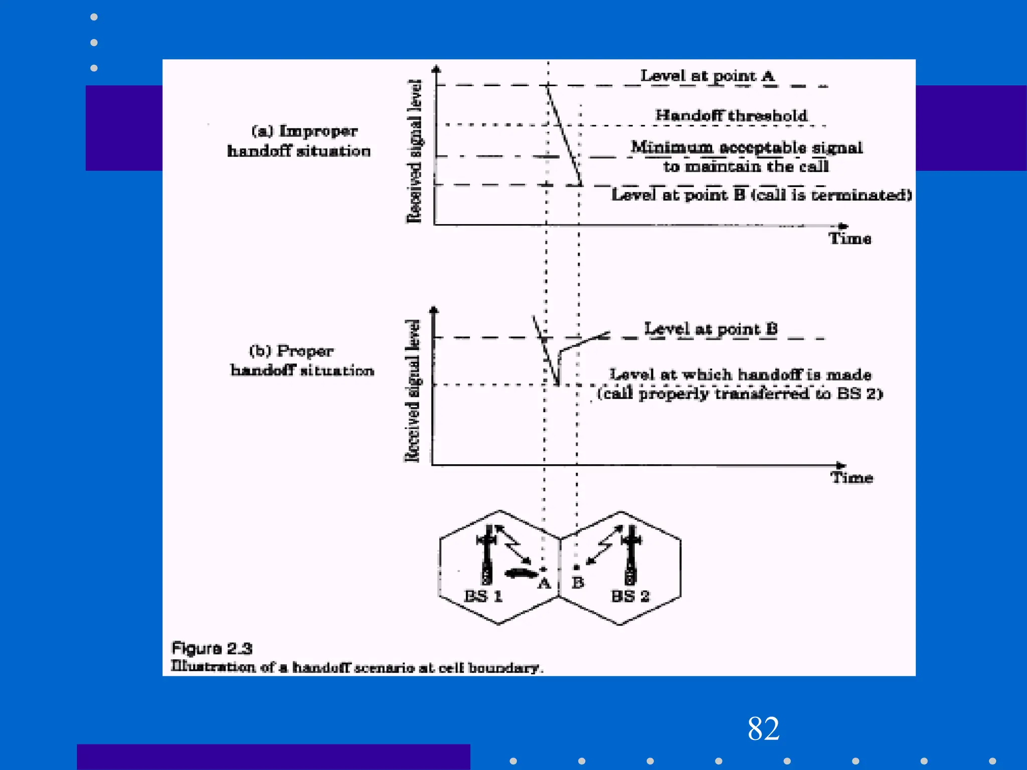
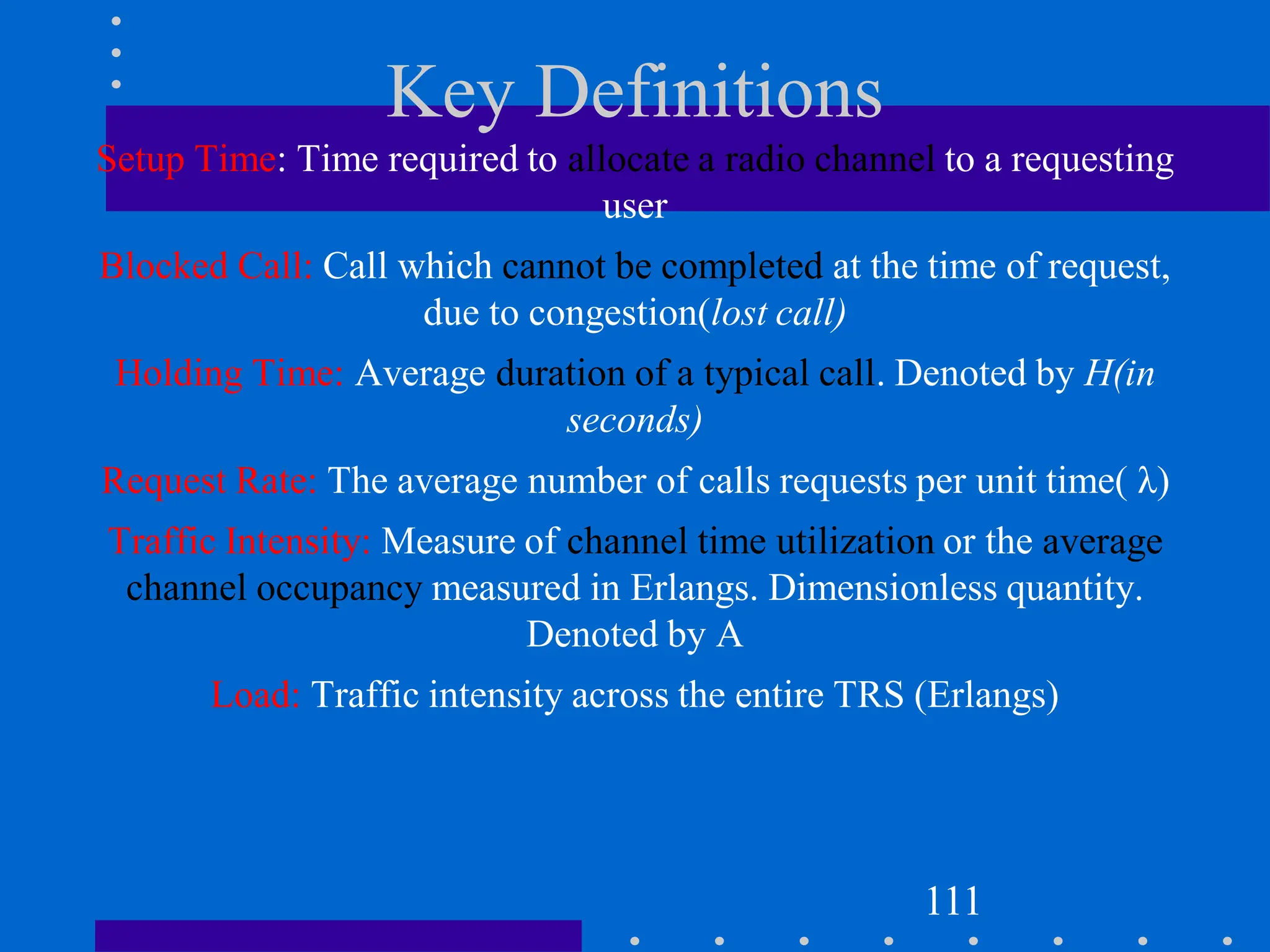
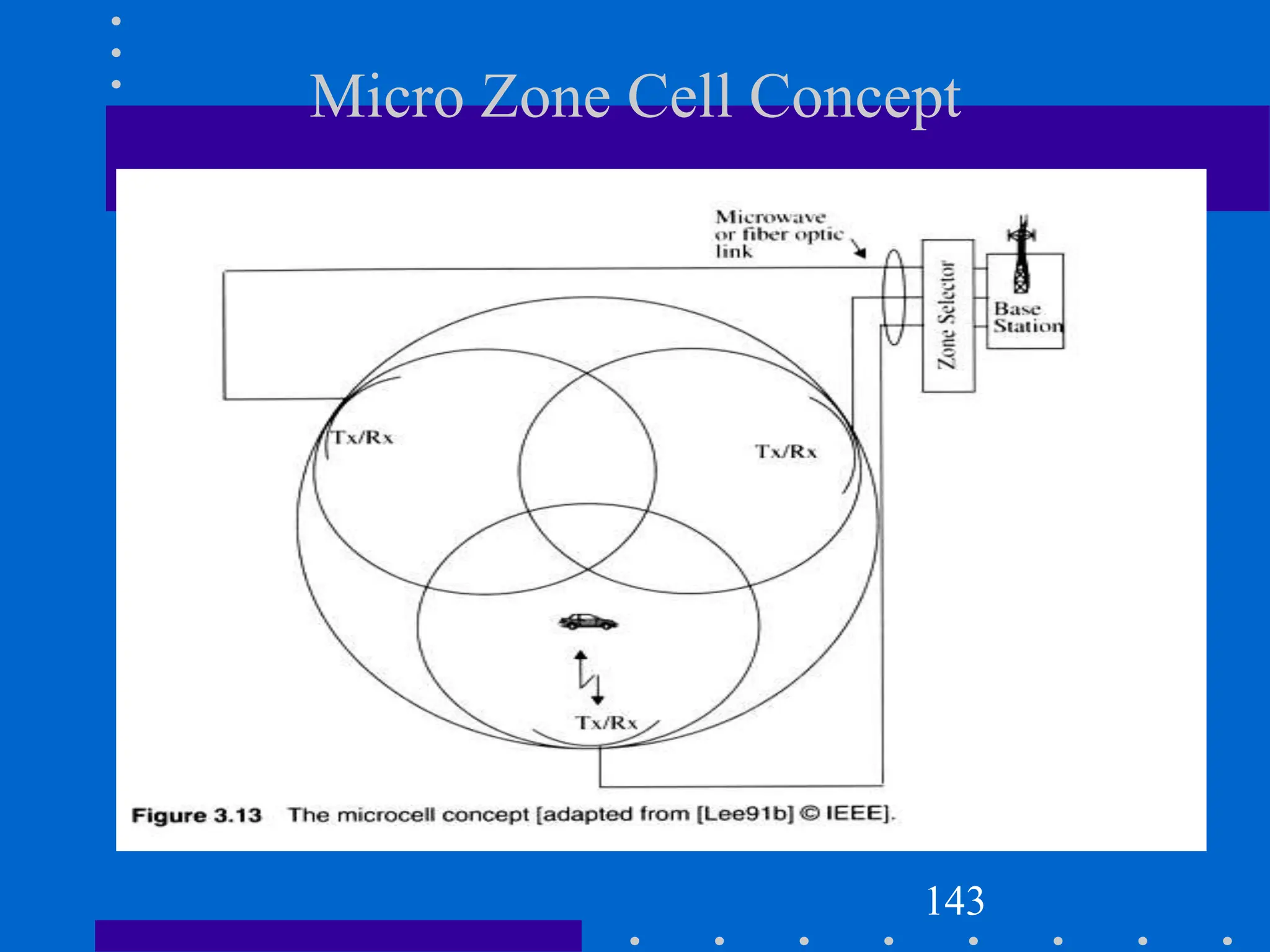
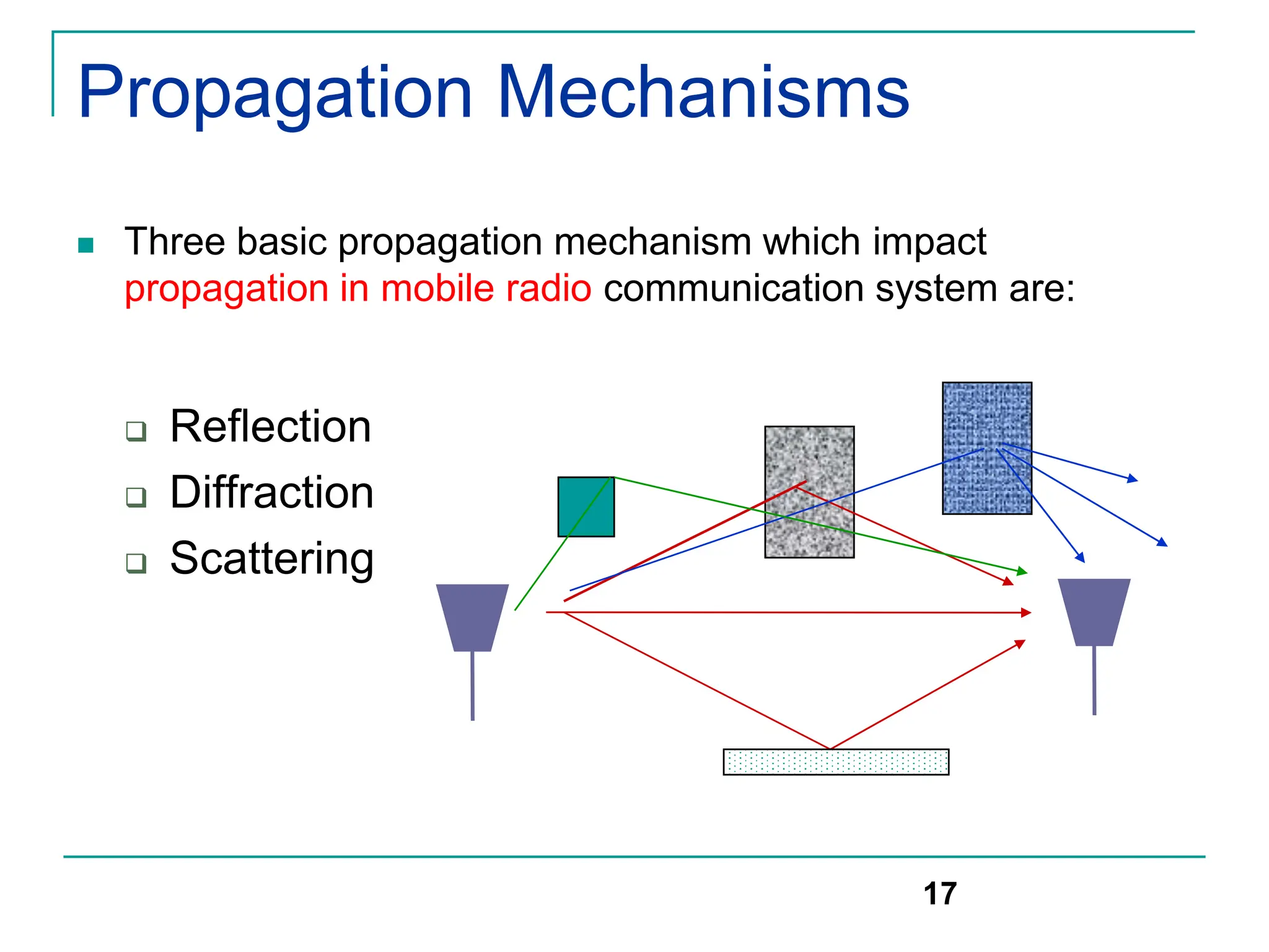
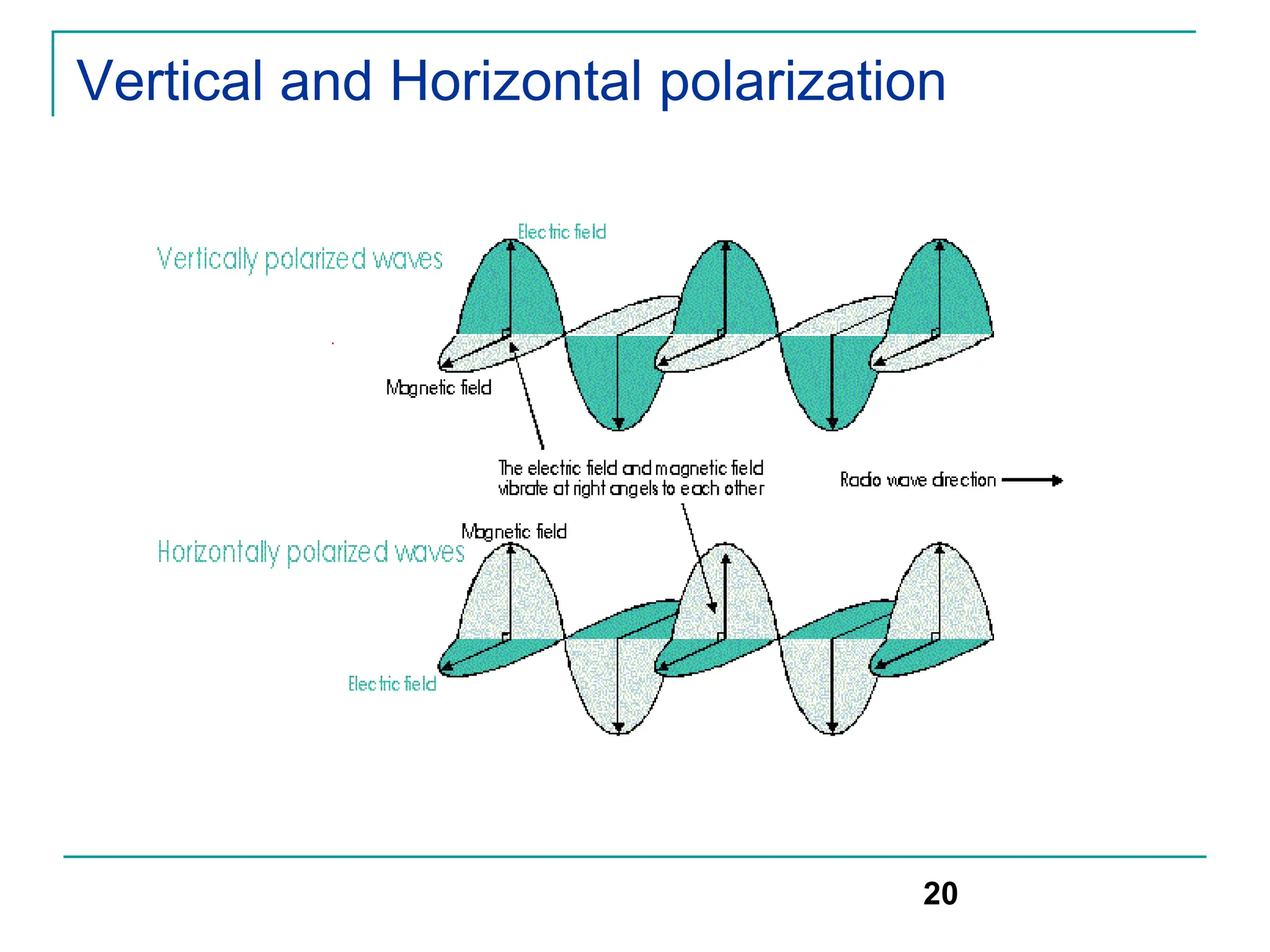
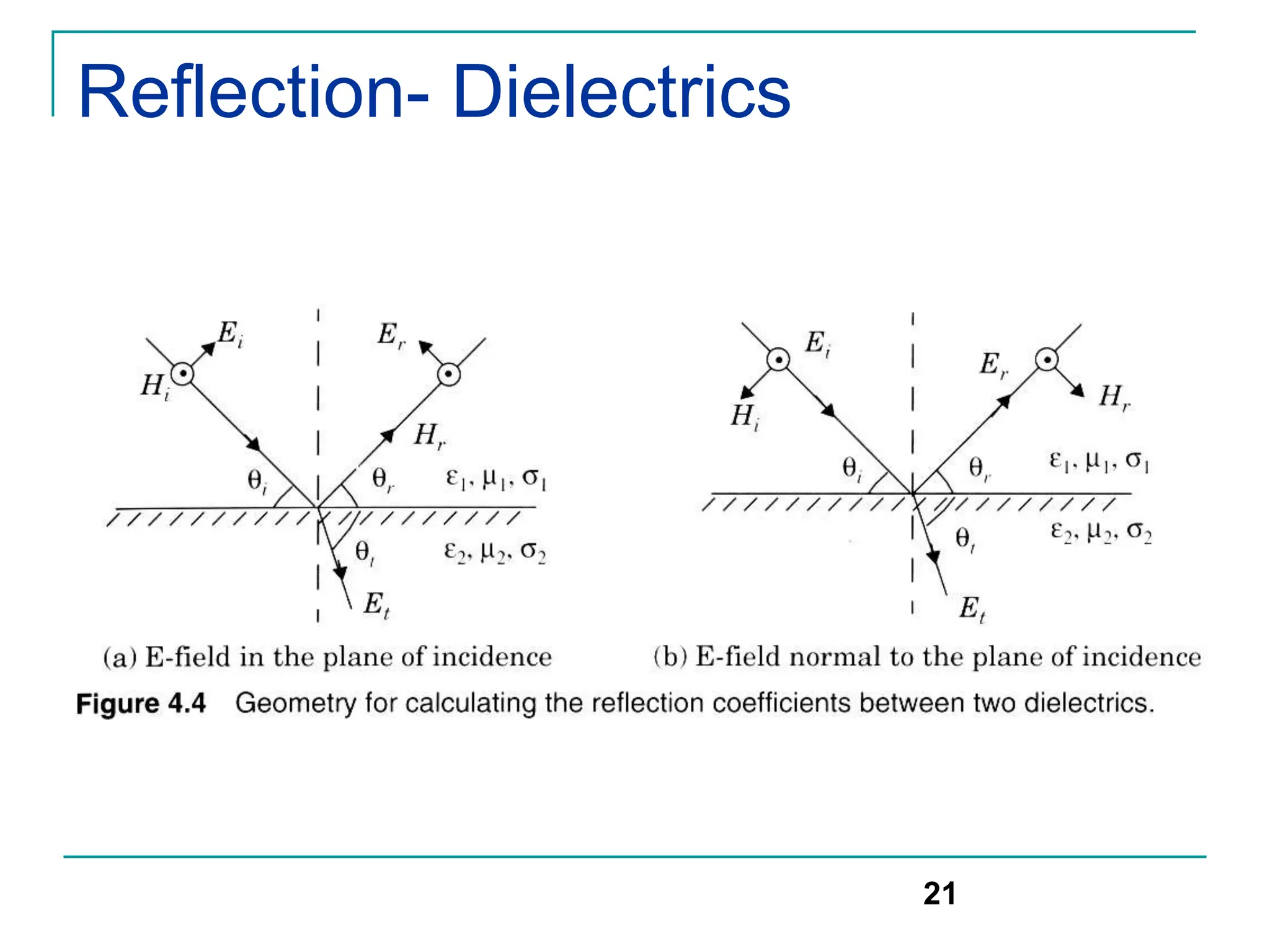
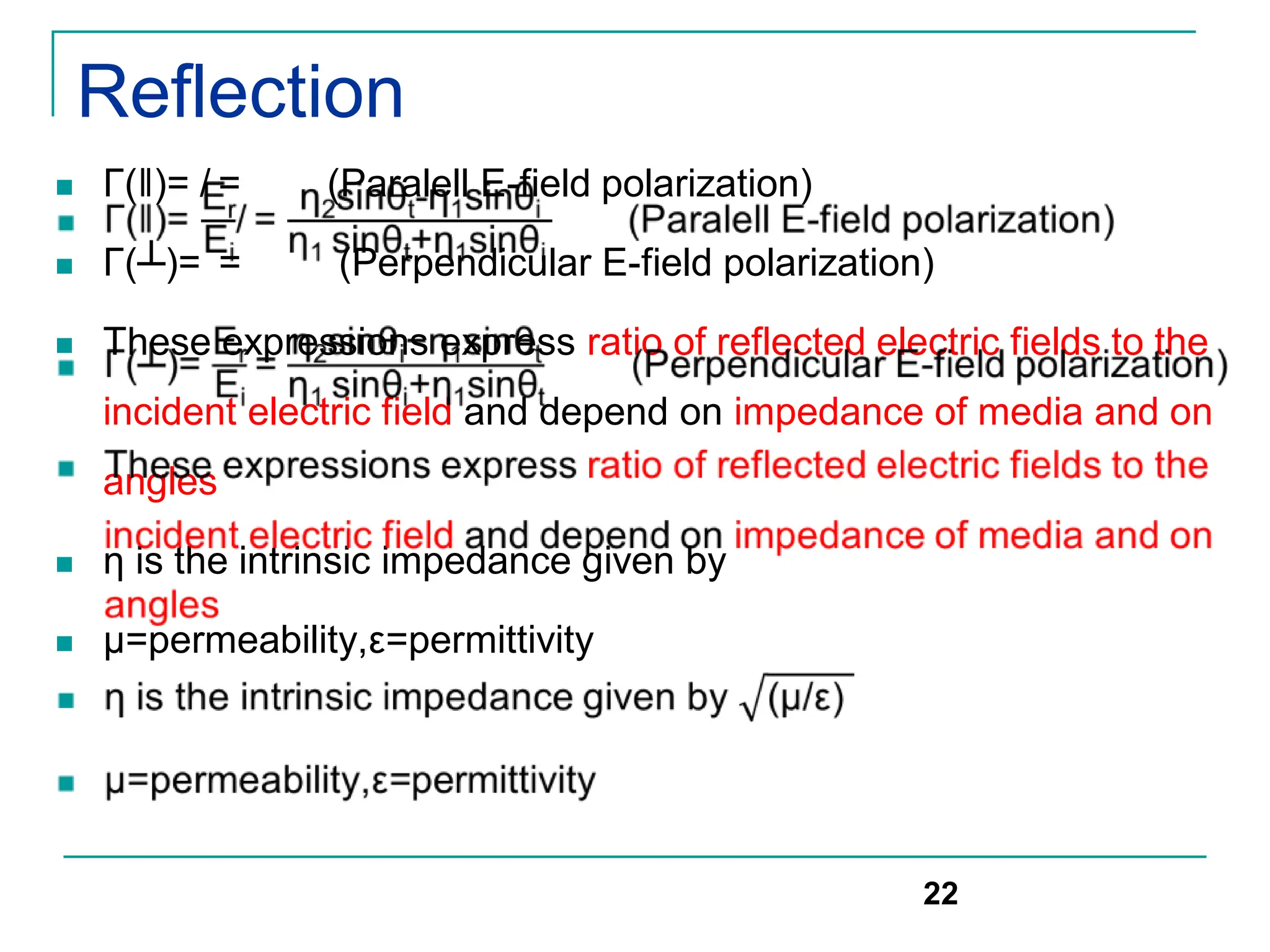
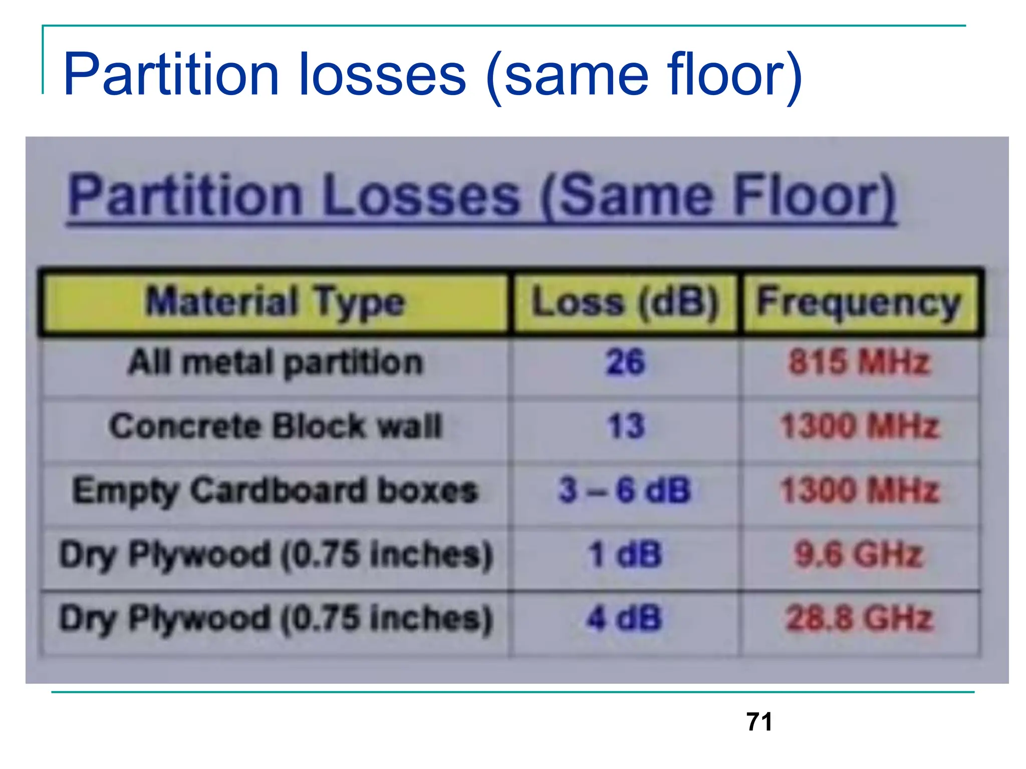
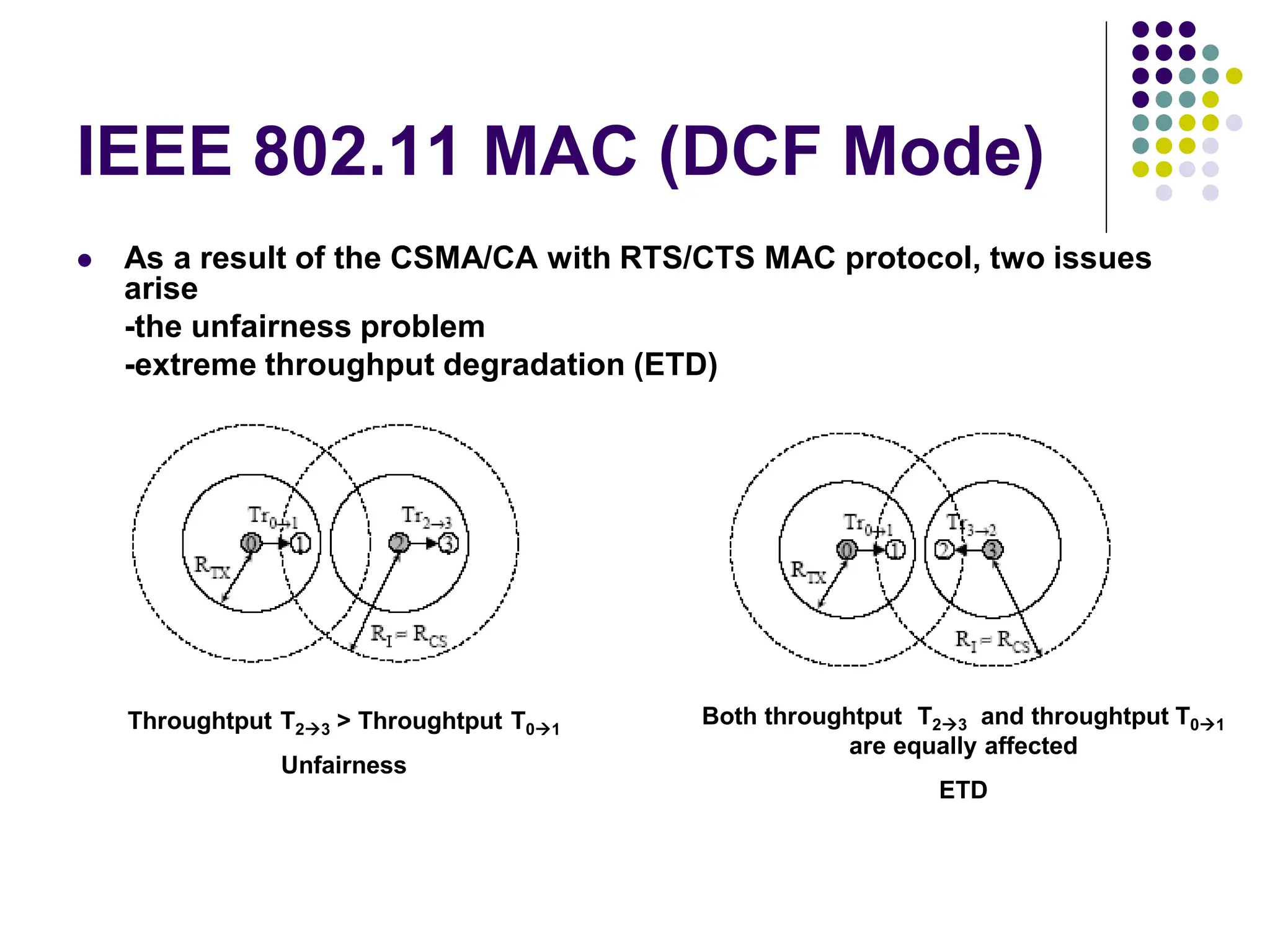
The document discusses mobile radio propagation, highlighting large-scale path loss and various propagation models crucial for wireless communication systems. It covers the properties of radio waves, their interaction with the environment (reflection, diffraction, and scattering), and notable models like the Longley-Rice and Okumura models for estimating signal strength and path loss. Additionally, it examines the impact of terrain and environment on signal propagation, providing a comprehensive overview of factors affecting wireless communication performance.


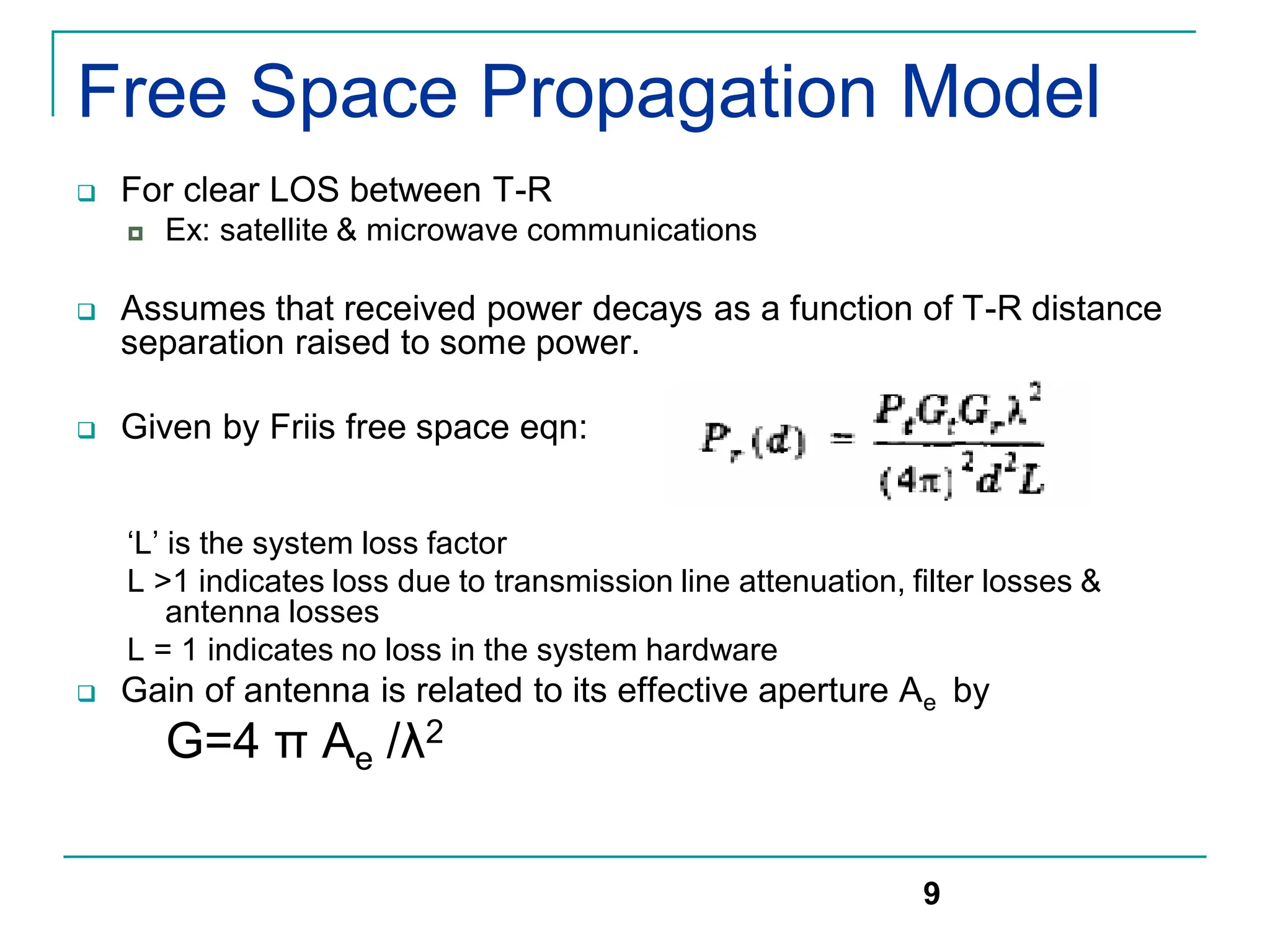

![Free Space Propagation Model
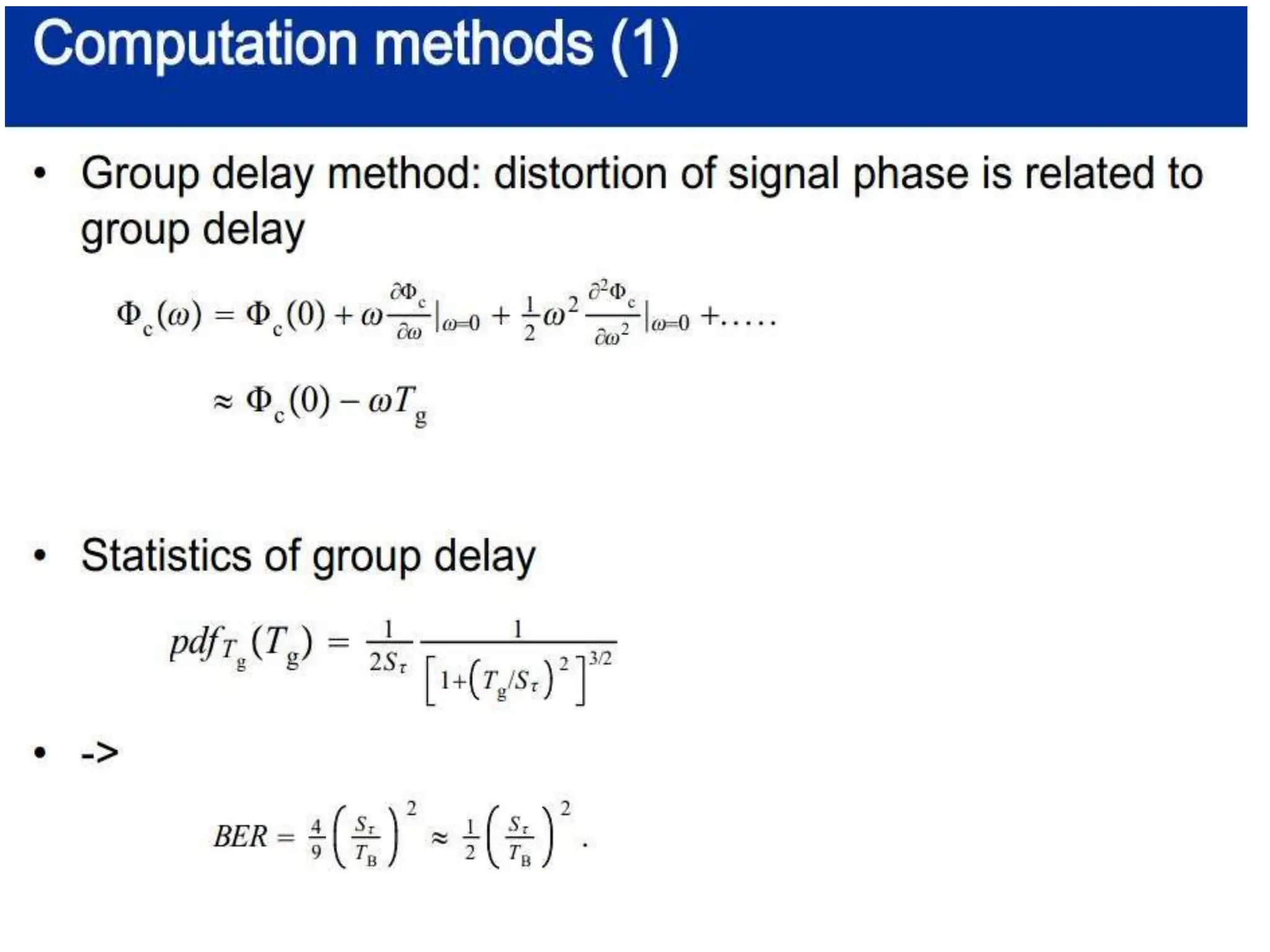
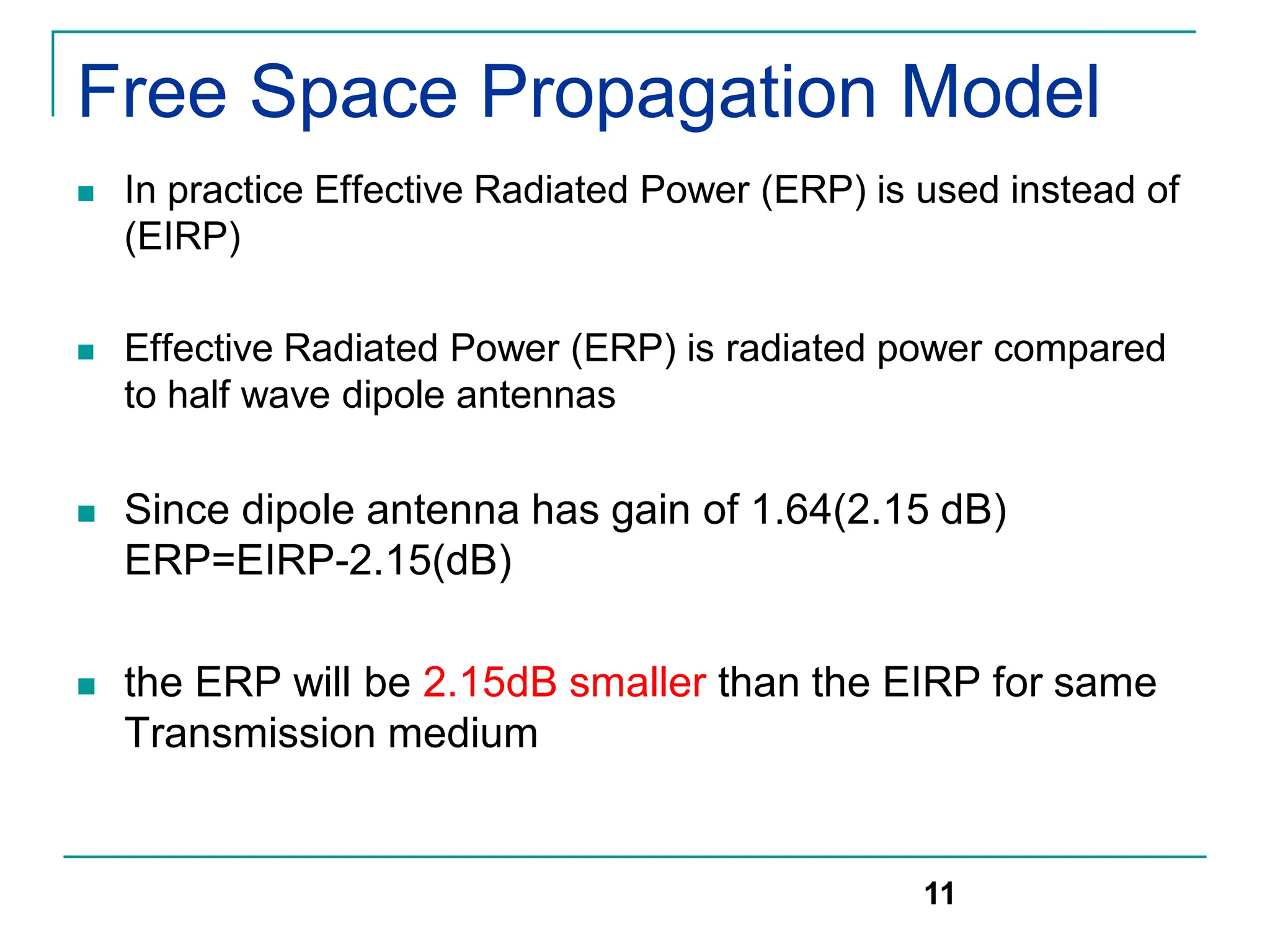
Path Loss (PL) represents signal attenuation and is defined
as difference between the effective transmitted power and
received power
Path loss PL(dB) = 10 log [Pt/Pr]
= -10 log {GtGr λ^2/(4π)^2d^2}
Without antenna gains (with unit antenna gains)
PL = - 10 log { λ^2/(4π)^2d^2}
Friis free space model is valid predictor for Pr for values of d
which are in the far-field of transmitting antenna
12](https://image.slidesharecdn.com/wcunit2-240913235922-2639a41d/75/wireless-communication-important-topics-12-2048.jpg)


![Numerical solution
An approximate numerical solution for
equation
Can be found using set of equations given
below for different values of v
41
[0,1]
20 log(0.5 e- 0.95v)
[-1,0]
20 log(0.5-0.62v)
> 2.4
20 log(0.225/v)
[1, 2.4]
20 log(0.4-(0.1184-(0.38-0.1v)2)1/2)
-1
0
v
Gd(dB)](https://image.slidesharecdn.com/wcunit2-240913235922-2639a41d/75/wireless-communication-important-topics-41-2048.jpg)


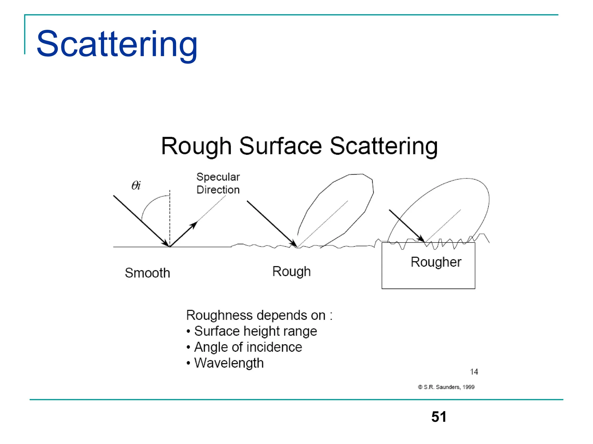
![Scattering
Rayleigh criterion: used for testing surface roughness
A surface is considered smooth if its min to max protuberance (bumps)
h is less than critical height hc
hc = λ/8 sinΘi
Scattering path loss factor ρs is given by
ρs =exp[-8[(π*σh *sinΘi)/ λ] 2]
Where h is surface height and σh is standard deviation of surface
height about mean surface height.
For rough surface, the flat surface reflection coefficient is multiplied by
scattering loss factor ρs to account for diminished electric field
Reflected E-fields for h> hc for rough surface can be calculated as
Гrough= ρsГ
50](https://image.slidesharecdn.com/wcunit2-240913235922-2639a41d/75/wireless-communication-important-topics-50-2048.jpg)


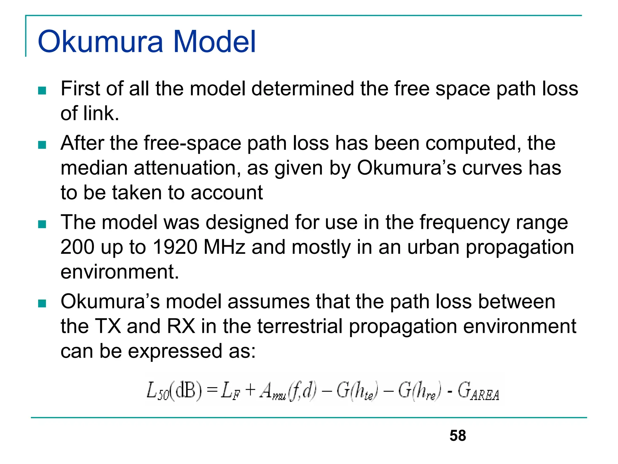

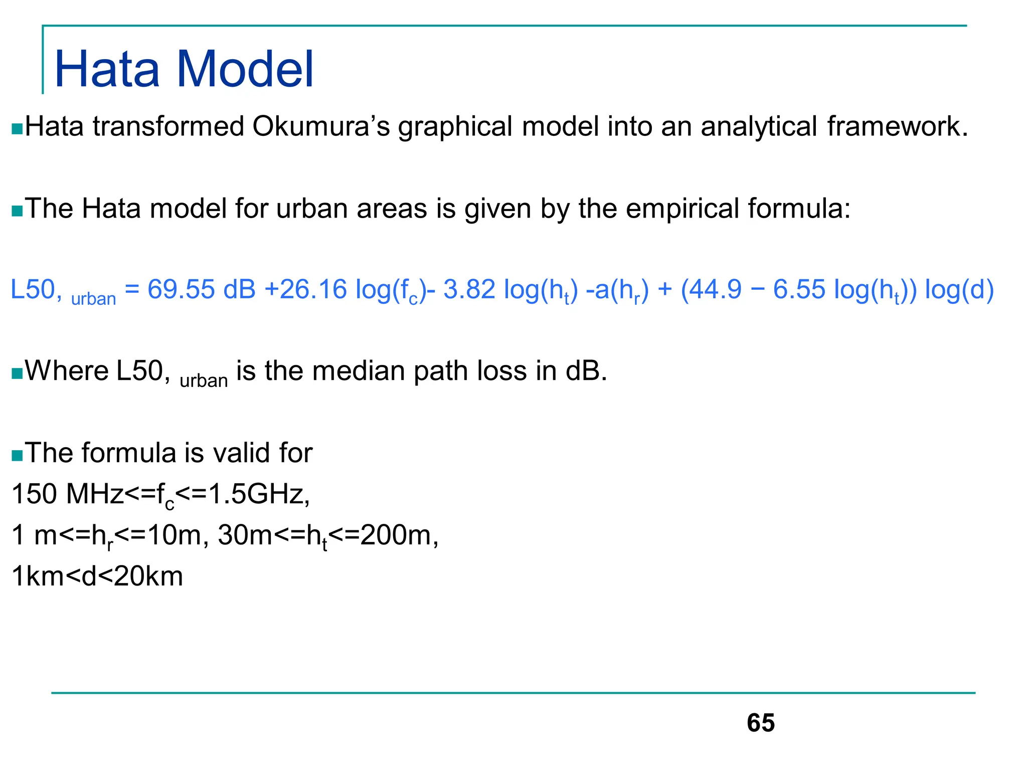
![Hata Model
The correction factor a(hr) for mobile antenna height hr for a small or
medium-sized city is given by:
a(hr) = (1.1 logfc − 0.7)hr − (1.56 log(fc) − 0.8) dB
For a large city it is given by
a(hr) = 8.29[log(1.54hr)]2 − 1.10 dB for fc <=300 MHz
3.20[log (11.75hr)]2 − 4.97 dB for fc >= 300 MHz
To obtain path loss for suburban area the standard Hata model is
modified as
L50 =L50(urban)-2[log(fc/28)]2-5.4
For rural areas
L50 =L50(urban)-4.78log(fc)2-18.33logfc -40.98
66](https://image.slidesharecdn.com/wcunit2-240913235922-2639a41d/75/wireless-communication-important-topics-66-2048.jpg)


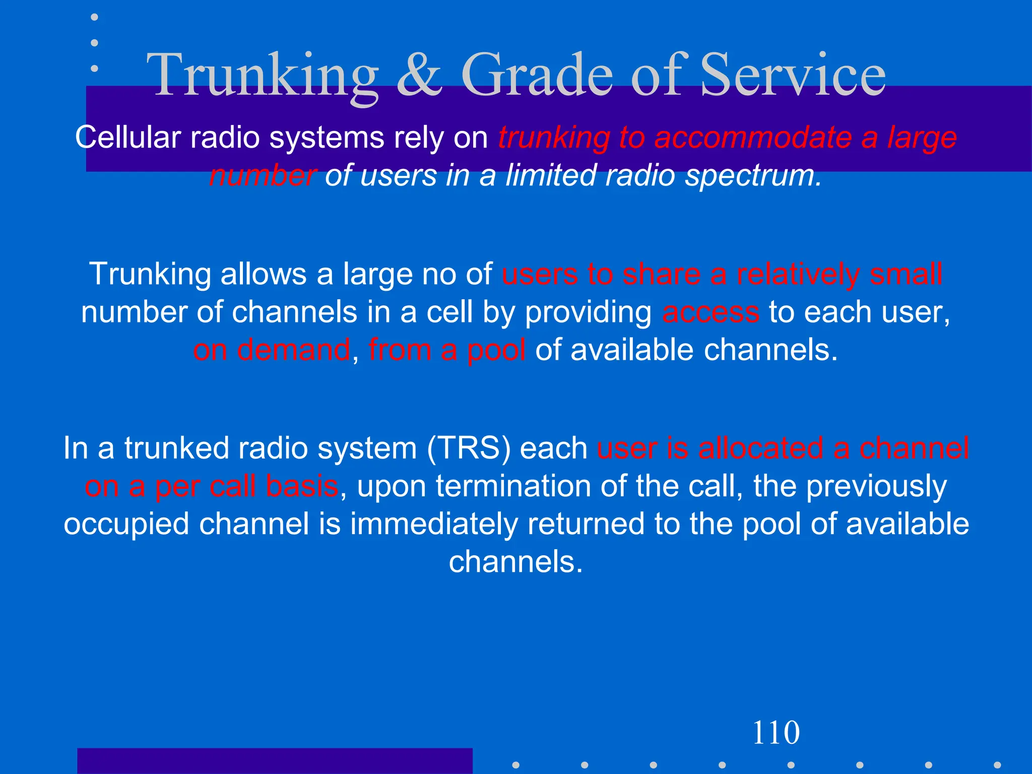
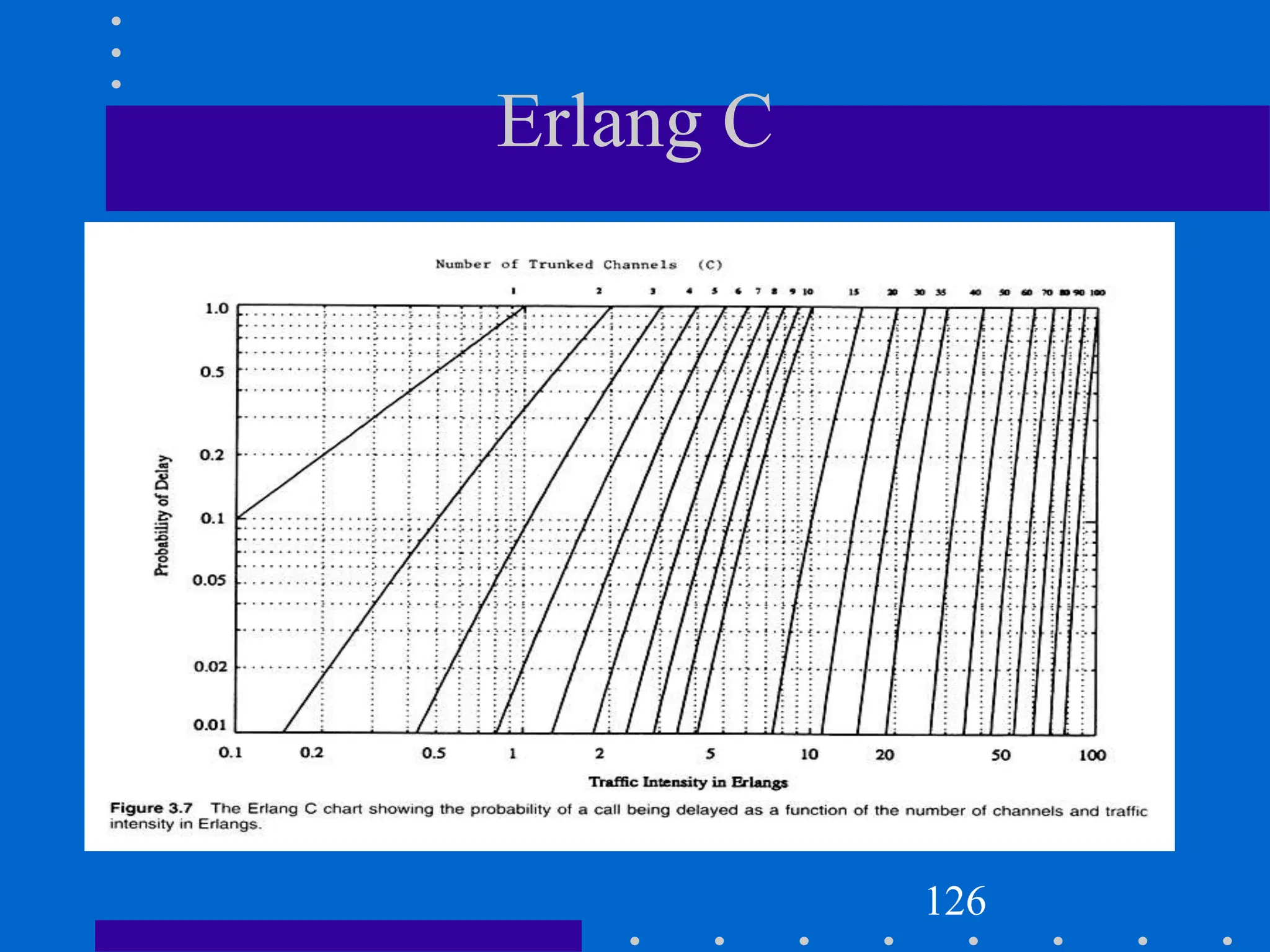
![Modeling of BCC Systems
Erlang B formula is given by
where C is the number of trunked channels offered by a trunked radio
system and A is the total offered traffic.
119
Pr[blocking]=
(AC/C ! )](https://image.slidesharecdn.com/wcunit2-240913235922-2639a41d/75/wireless-communication-important-topics-229-2048.jpg)
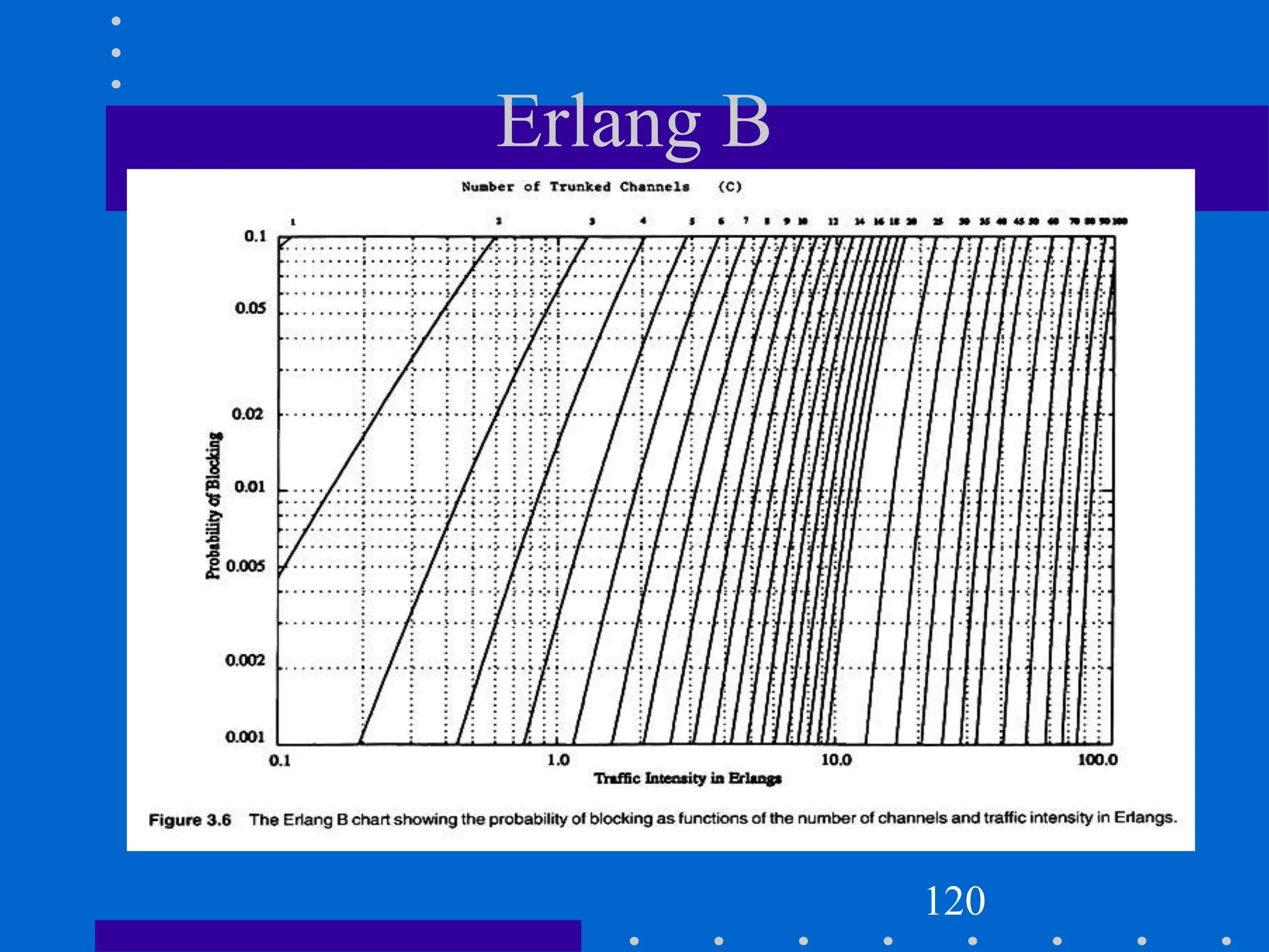
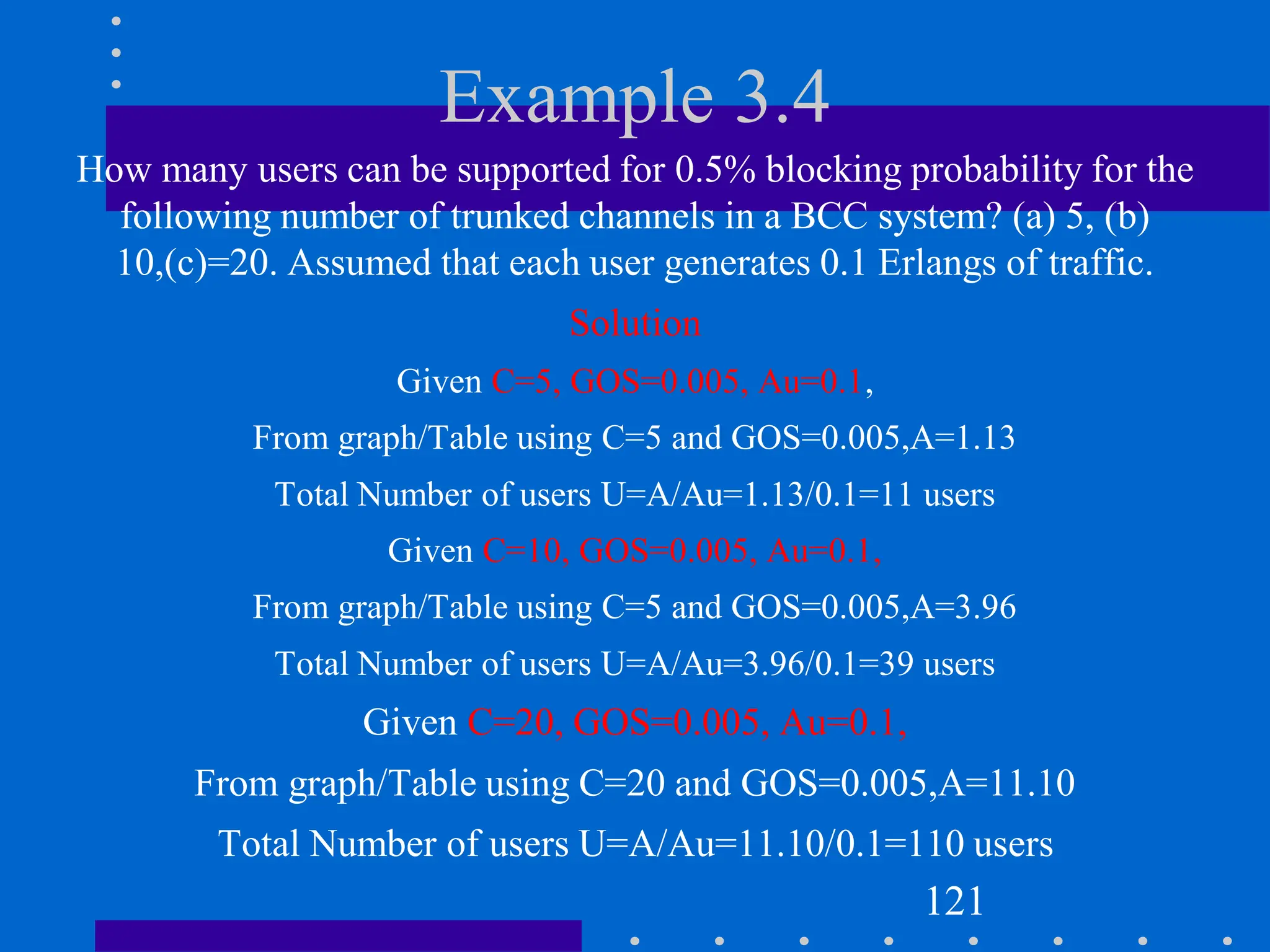
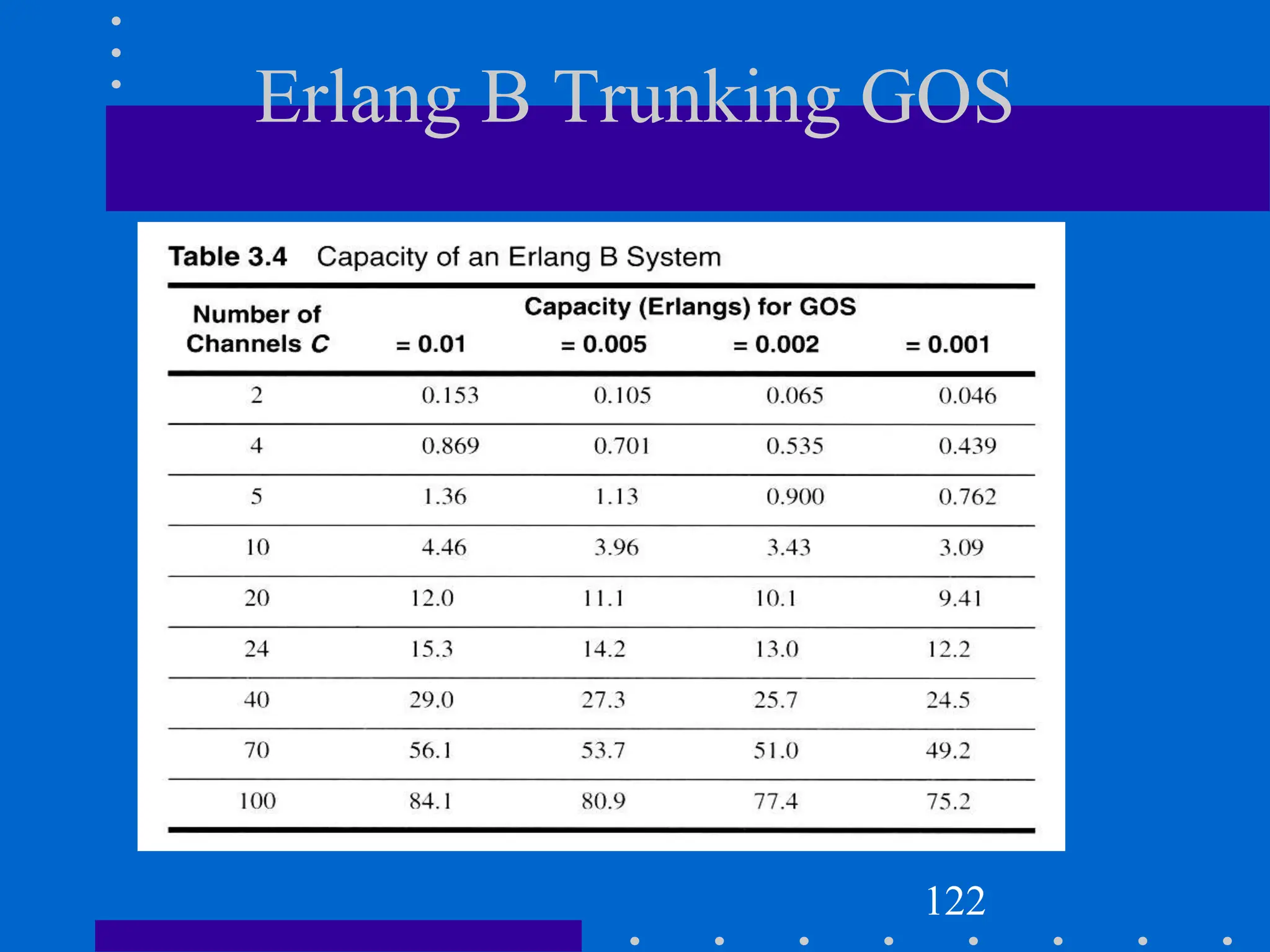
![BCC System Example
Assuming that each user in a system generates a traffic intensity of 0.2
Erlangs, how many users can be supported for 0.1% probability of
blocking in an Erlang B system for a number of trunked channels equal
to 60.
Solution 1:
System is an Erlang B
Au = 0.2 Erlangs
Pr [Blocking] = 0.001
C = 60 Channels
From the Erlang B figure, we see that
A ≈ 40 Erlangs
Therefore U=A/Au=40/0.02=2000users.
123](https://image.slidesharecdn.com/wcunit2-240913235922-2639a41d/75/wireless-communication-important-topics-233-2048.jpg)
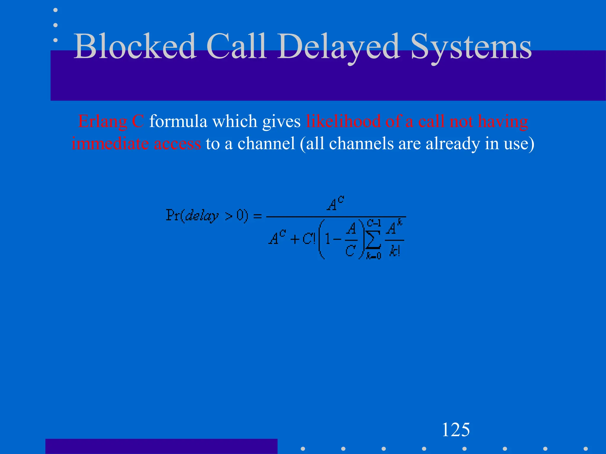
![Modeling of BCD Systems
Probability that any caller is delayed in queue for a wait time greater
than t seconds is given as GOS of a BCD System
The probability of a call getting delayed for any period of time greater
than zero is
P[delayed call is forced to wait > t sec]=P[delayed] x Conditional P[delay
is >t sec]
Mathematically;
Pr[delay>t] = Pr [delay>0] Pr [delay>t| delay>0]
Where P[delay>t| delay>0]= e(-(C-A)t/H)
Pr[delay>t] = Pr [delay>0] e(-(C-A)t/H)
where C = total number of channels, t =delay time of interest, H=average
duration of call
127](https://image.slidesharecdn.com/wcunit2-240913235922-2639a41d/75/wireless-communication-important-topics-237-2048.jpg)
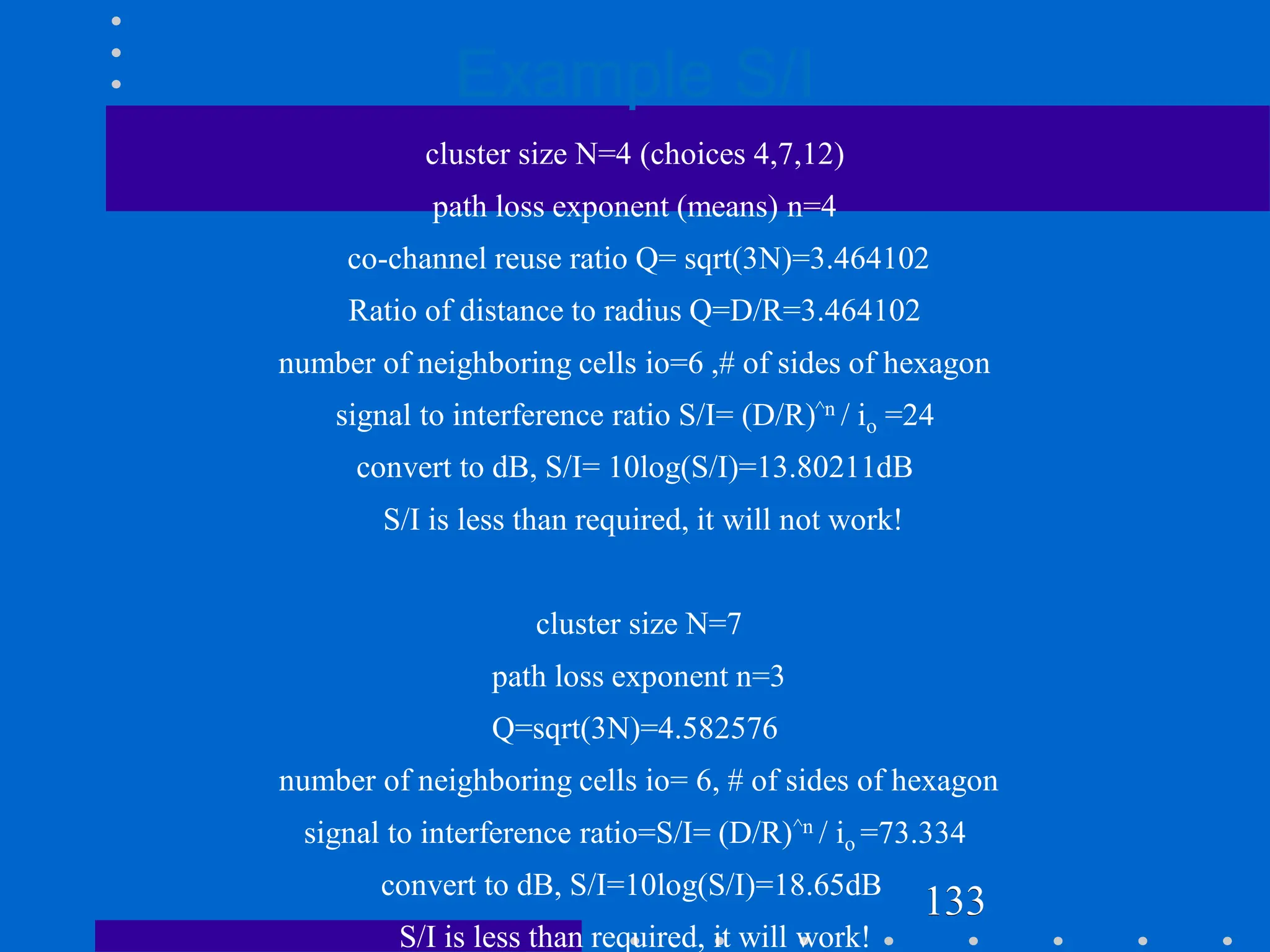
![Cell Splitting-Power Issues
Suppose the cell radius of new cells is reduced by half
What is the required transmit power for these new cells??
Pr[at old cell boundary]=Pt1R-n
Pr[at new cell boundary]= Pt2(R/2) –n
where Pt1and Pt2are the transmit powers of the larger and smaller cell
base stations respectively, and n is the path loss exponent.
So, Pt2= Pt1/2n
If we take n=3 and the received powers equal to each other, then
Pt2=Pt1/8
In other words, the transmit power must be reduced by 9dB in order to fill in
the original coverage area while maintaining the S/I requirement
134](https://image.slidesharecdn.com/wcunit2-240913235922-2639a41d/75/wireless-communication-important-topics-244-2048.jpg)


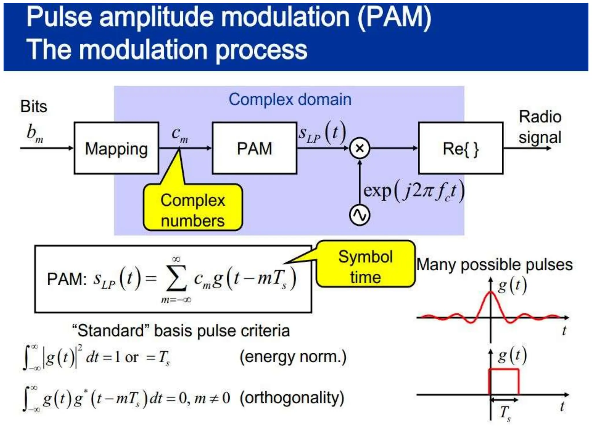
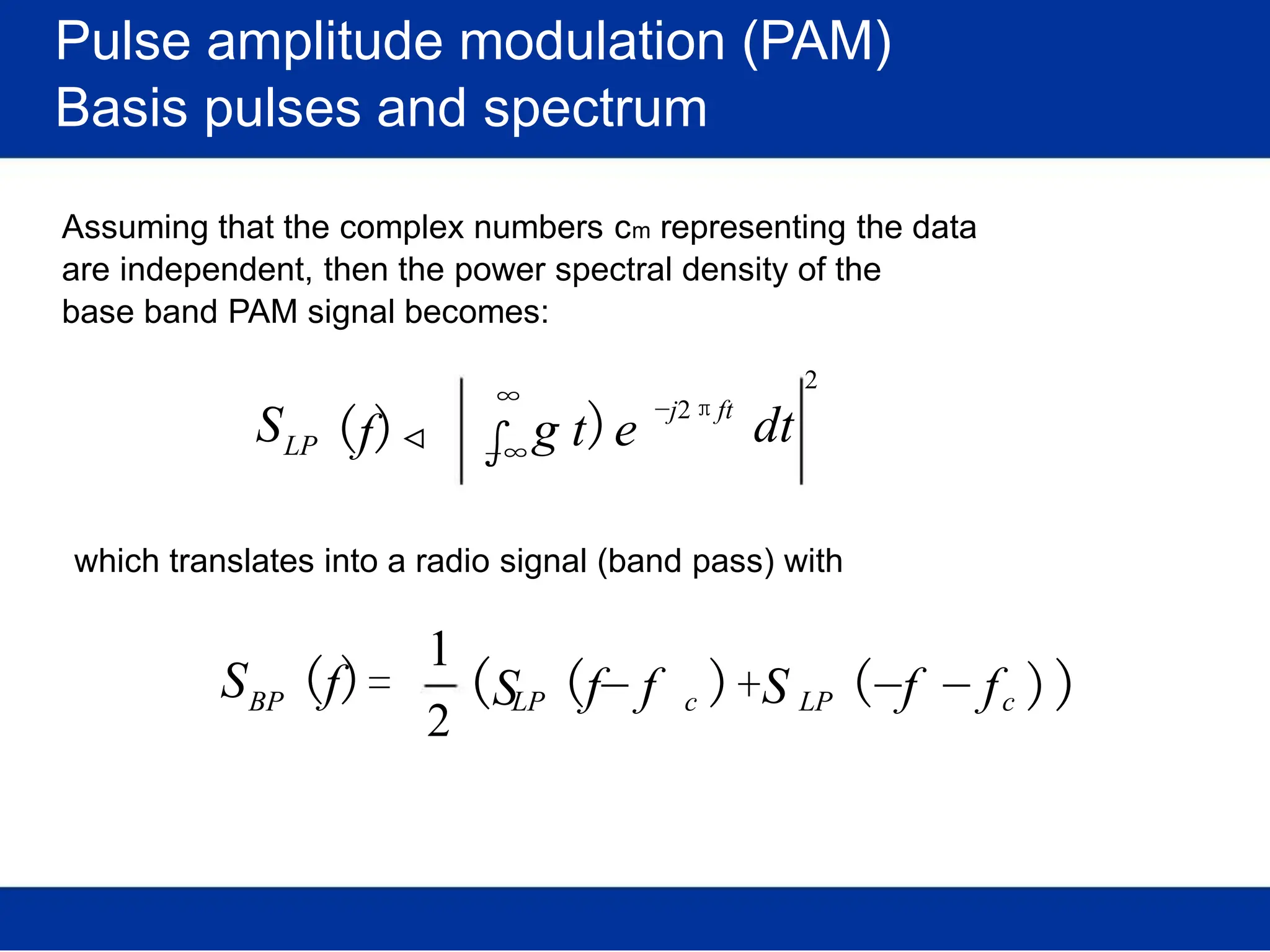
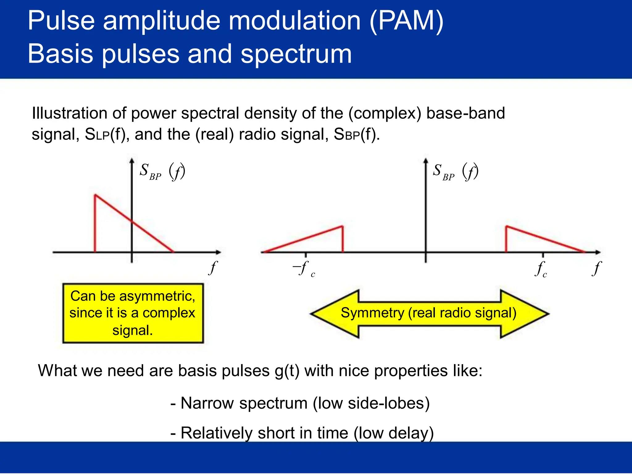
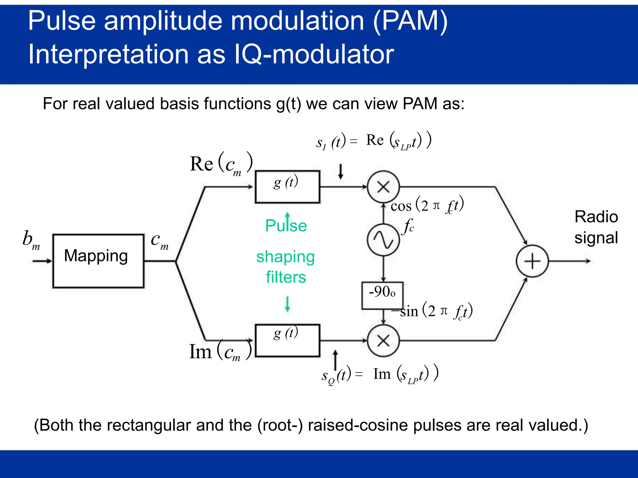
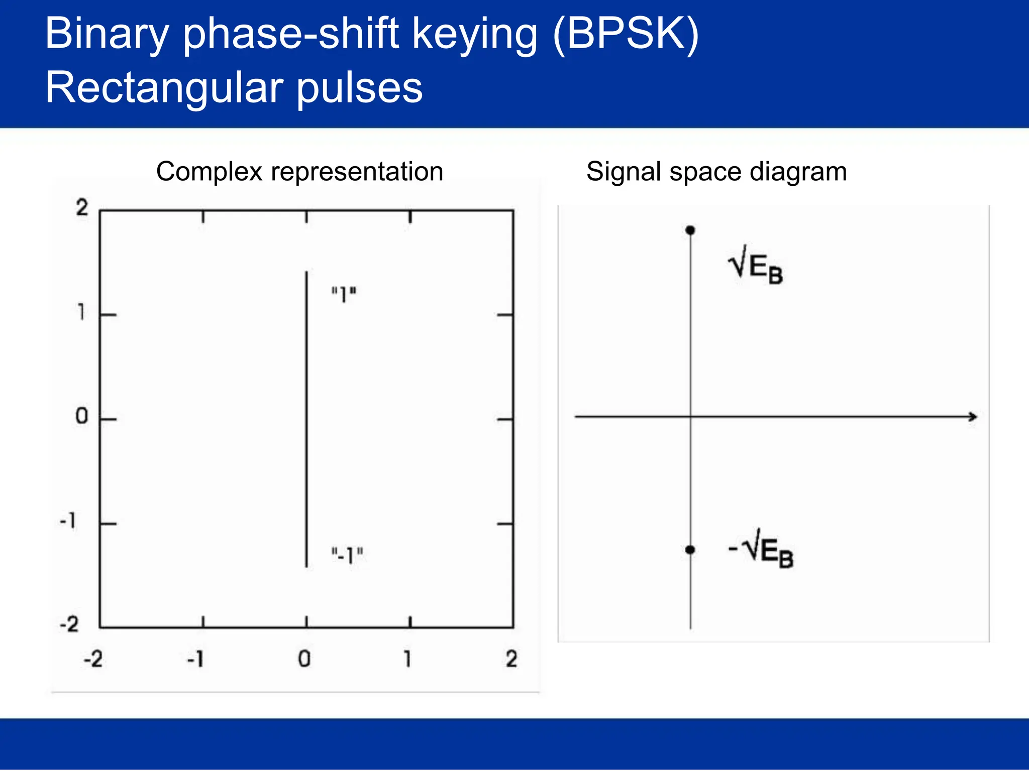
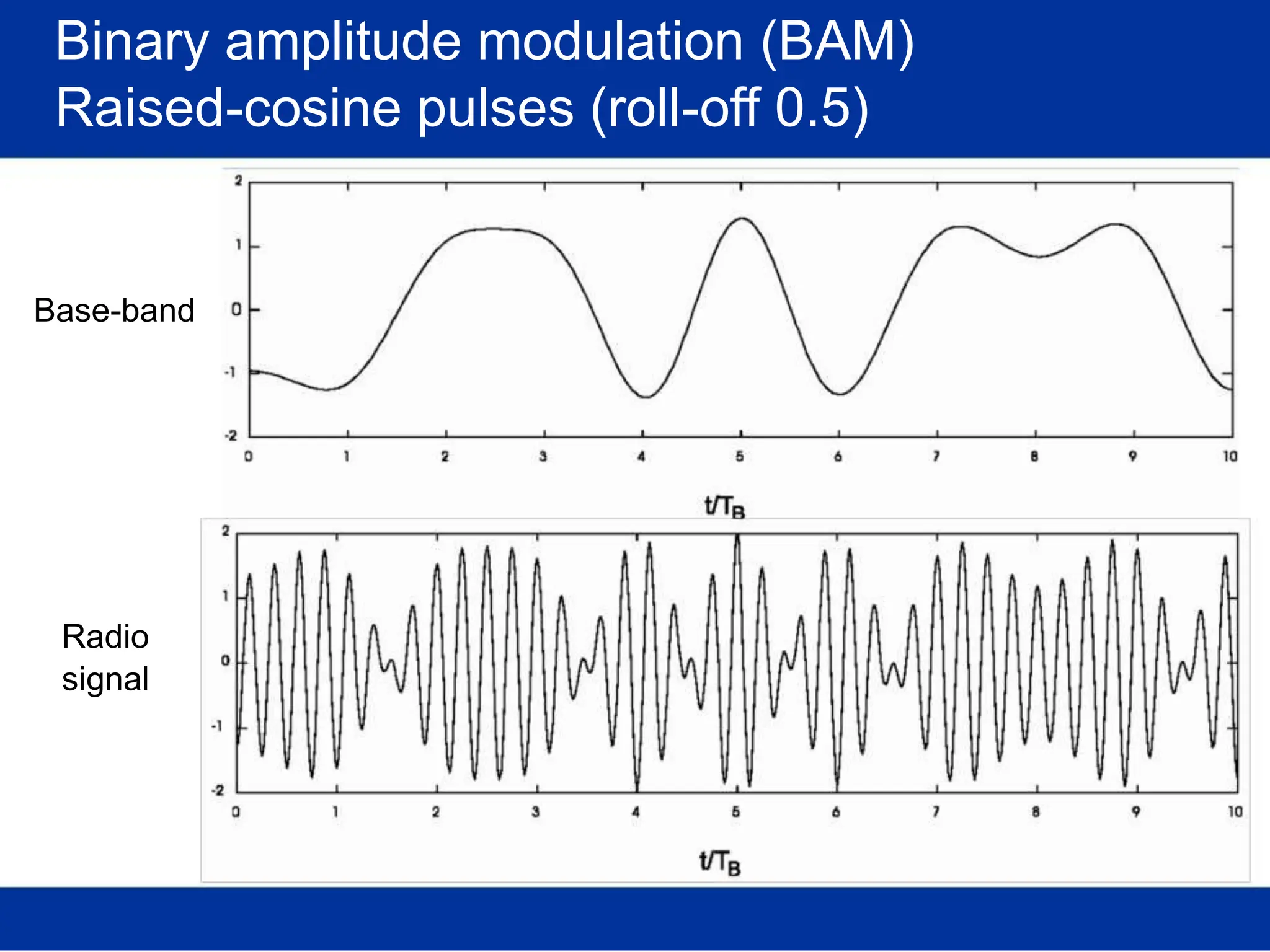
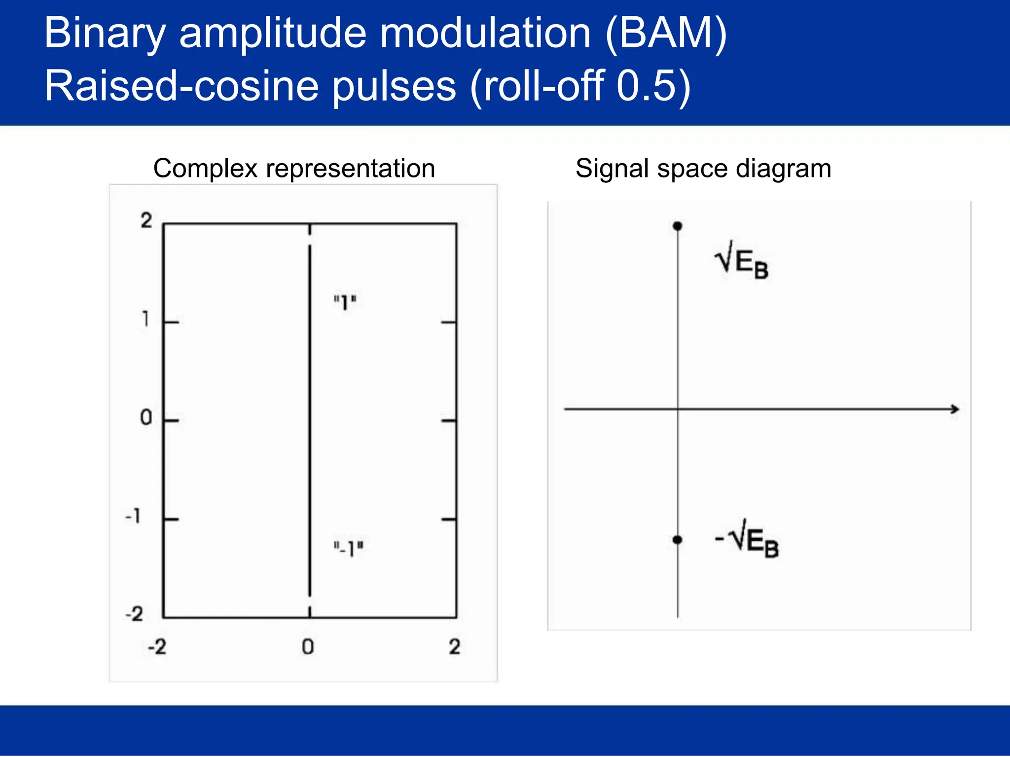
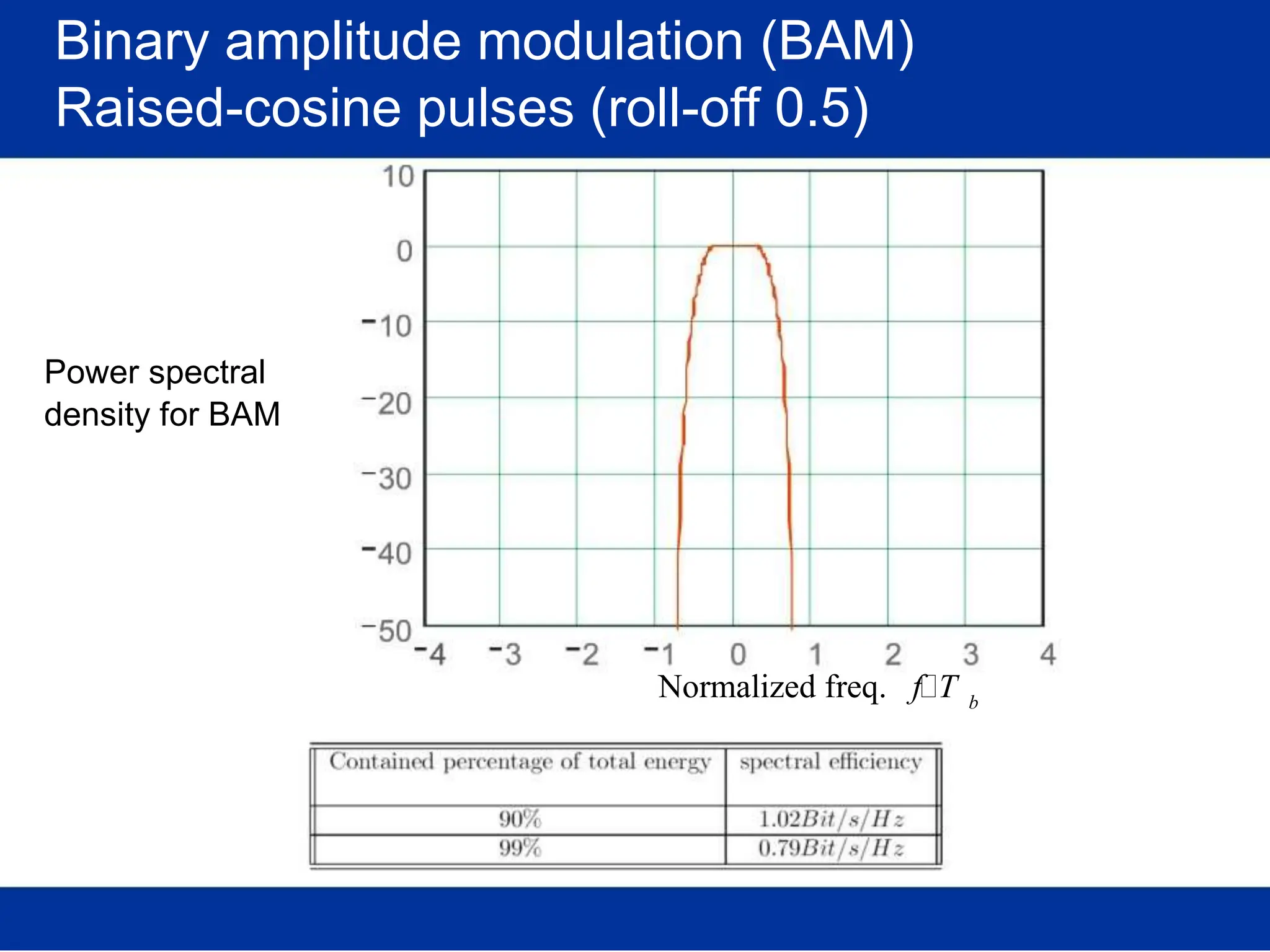
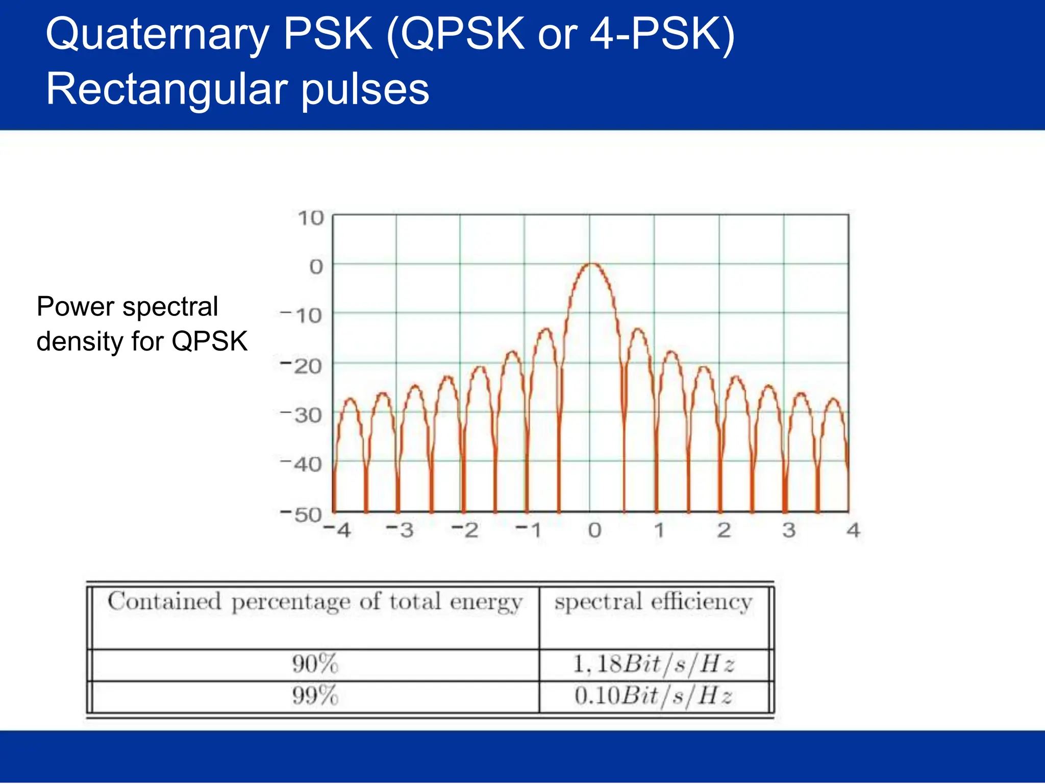
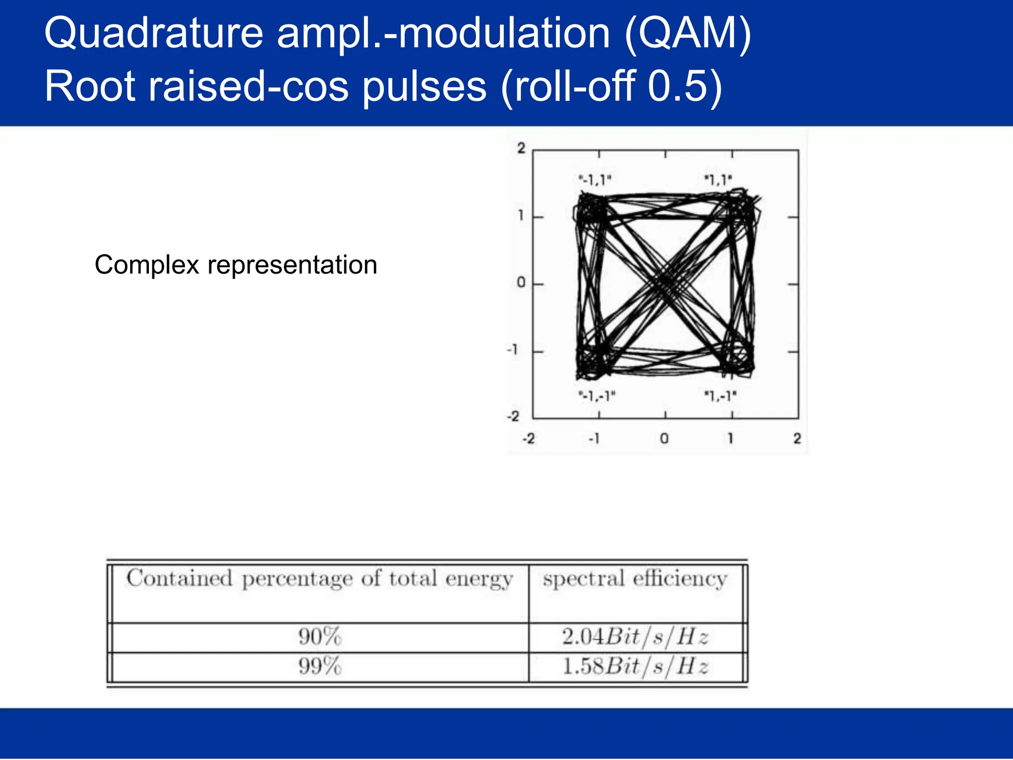
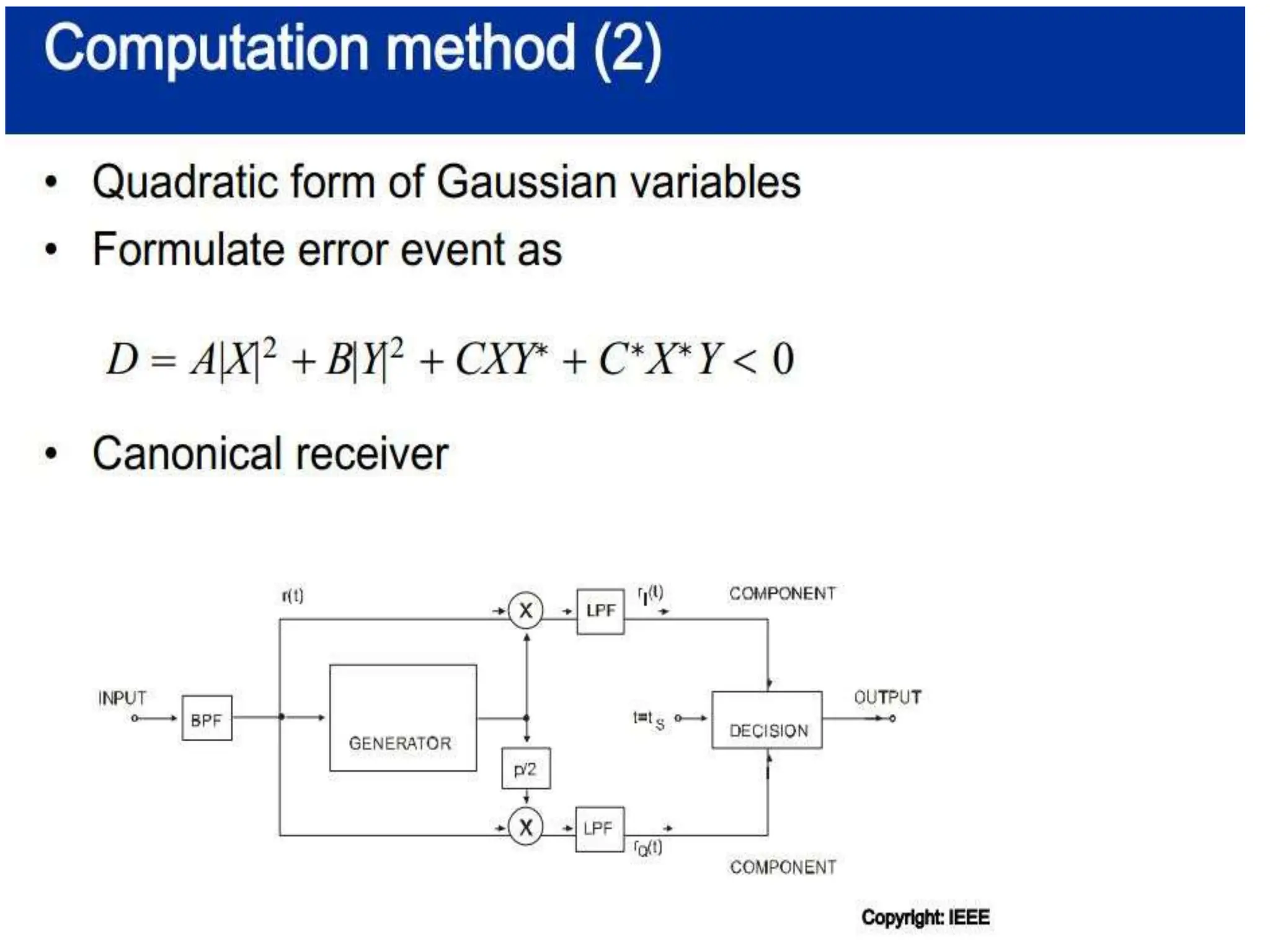
![Pulse amplitude modulation (PAM)
Basis pulses
TIME DOMAIN
Normalized time t
FREQ. DOMAIN
Rectangular [in time]
/T Normalized freq. f/T
s s
(Root-) Raised-cosine [in freq.]
Normalized time t /T Normalized freq. f/T
s s](https://image.slidesharecdn.com/wcunit2-240913235922-2639a41d/75/wireless-communication-important-topics-270-2048.jpg)


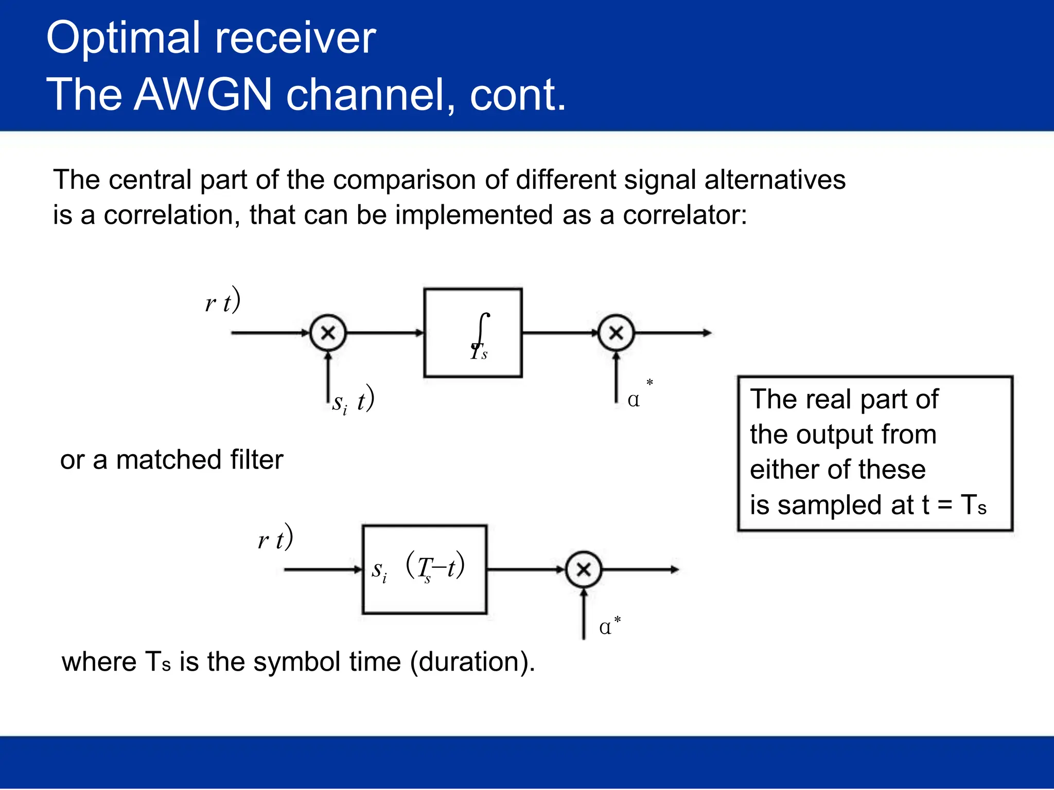
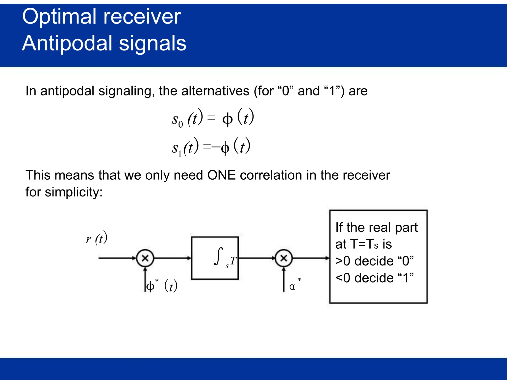
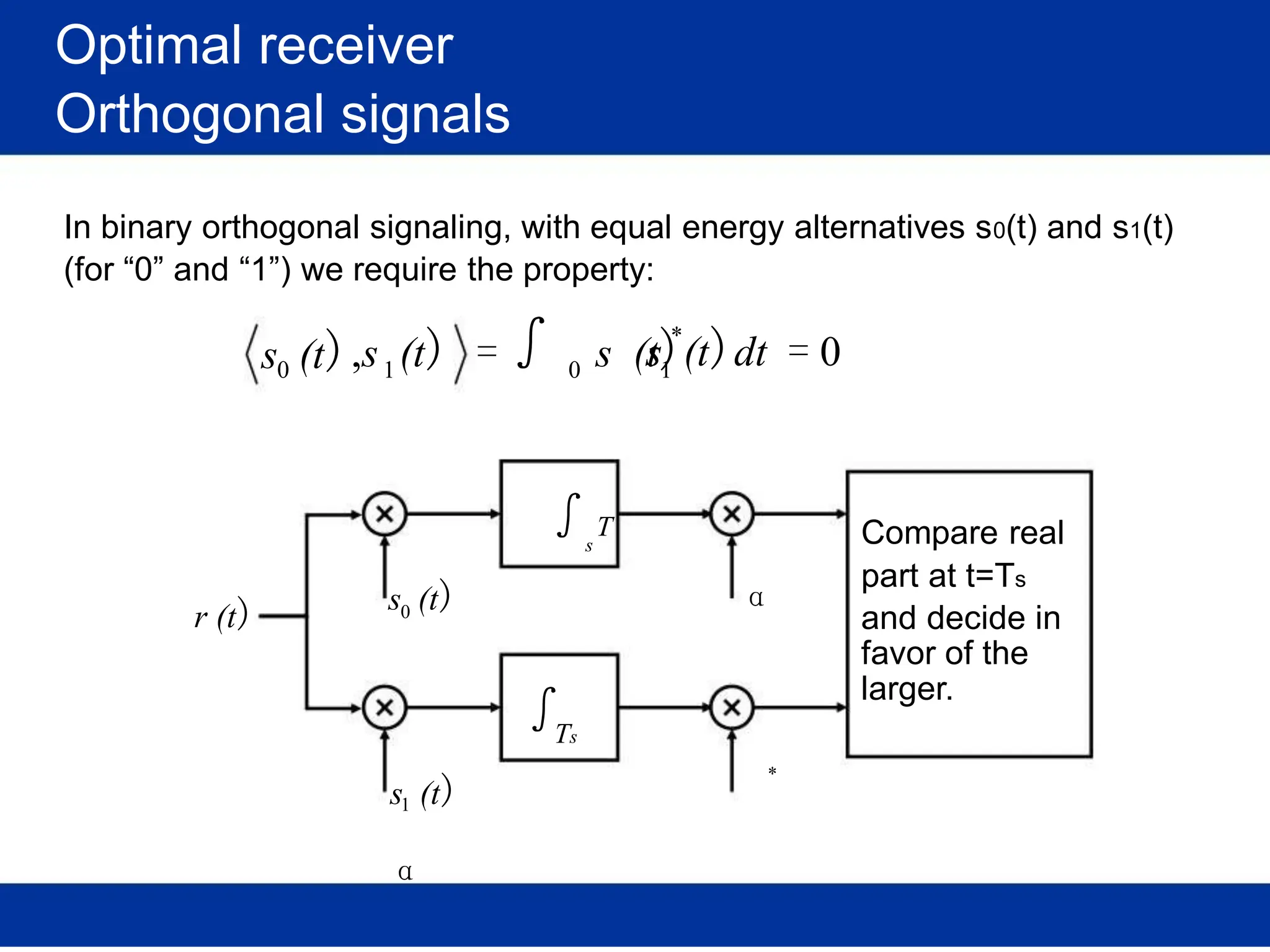
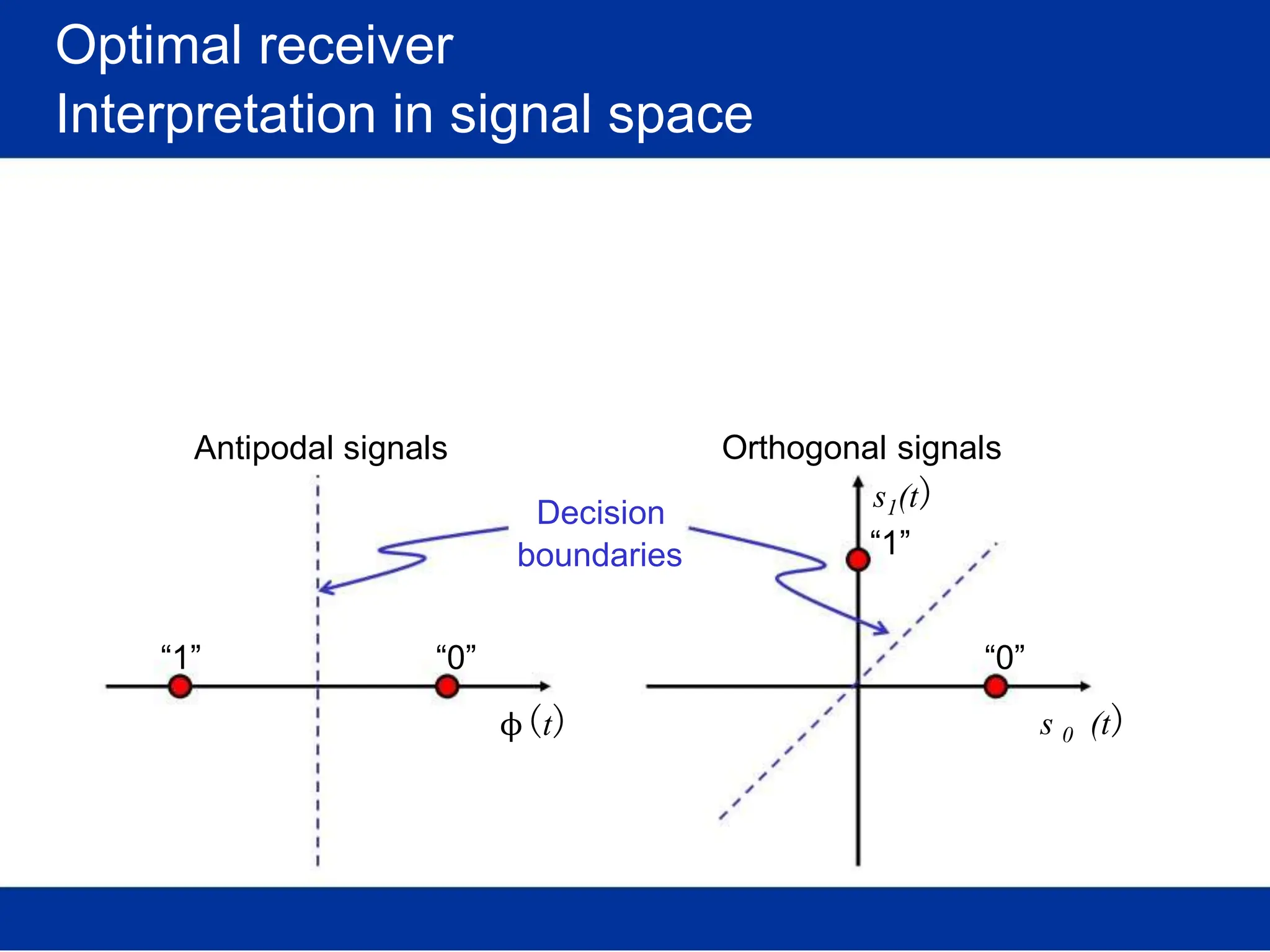
![Optimal receiver
Bit-error rates (BER), cont.
100
2PAM/4QAM
10-1
10-2
10-3
10-4
10-5
10-6
0 2 4 6
8PSK
16QAM
8 10 12 14 16 18 20
E /N [dB]
b 0](https://image.slidesharecdn.com/wcunit2-240913235922-2639a41d/75/wireless-communication-important-topics-321-2048.jpg)
![Optimal receiver
Where do we get Eb and N0?
Where do those magic numbers Eb and N0 come from?
The noise power spectral density N0 is calculated according to
N0 = kTF ⇔N
0 0 0|dB =−204+F 0|dB
where F0 is the noise factor of the “equivalent” receiver noise source.
The bit energy Eb can be calculated from the received
power C (at the same reference point as N0). Given a certain
data-rate db [bits per second], we have the relation
Eb
=C/ d b ⇔E =C −d
b|dB |dB b|dB
THESE ARE THE EQUATIONS THAT RELATE DETECTOR
PERFORMANCE ANALYSIS TO LINK BUDGET CALCULATIONS!](https://image.slidesharecdn.com/wcunit2-240913235922-2639a41d/75/wireless-communication-important-topics-323-2048.jpg)
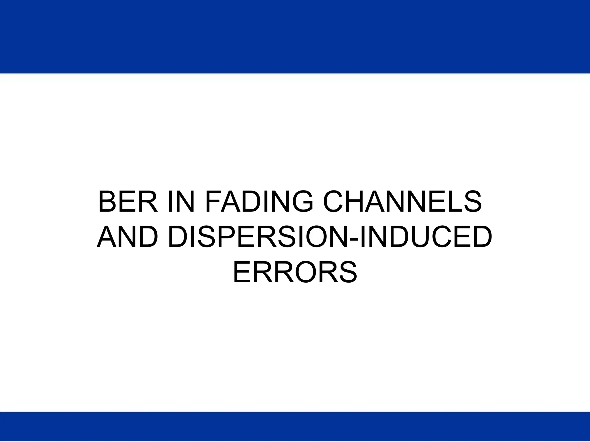
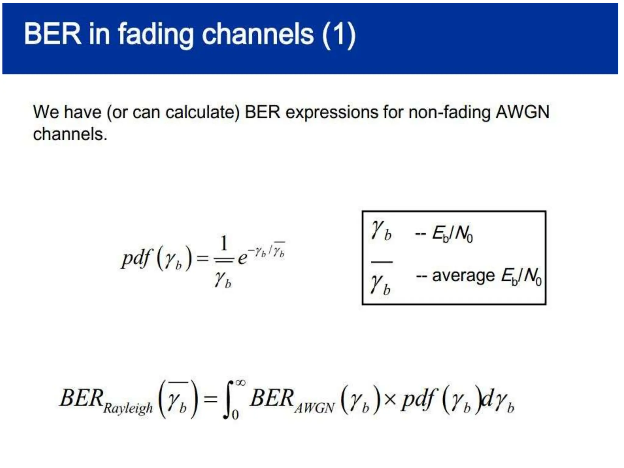
![BER in fading channels (2)
THIS IS A SERIOUS PROBLEM!
Bit error rate (4QAM)
100
10 dB Rayleigh fading
10-1
10 x
10-2
10-3
10-4
10-5 No fading
10-6
0 2 4 6 8 10 12 14 16 18 20
Eb/N0 [dB]](https://image.slidesharecdn.com/wcunit2-240913235922-2639a41d/75/wireless-communication-important-topics-329-2048.jpg)


![Free Space Propagation Model
Path Loss (PL) represents signal attenuation and is defined
as difference between the effective transmitted power and
received power
Path loss PL(dB) = 10 log [Pt/Pr]
= -10 log {GtGr λ^2/(4π)^2d^2}
Without antenna gains (with unit antenna gains)
PL = - 10 log { λ^2/(4π)^2d^2}
Friis free space model is valid predictor for Pr for values of d
which are in the far-field of transmitting antenna
12](https://image.slidesharecdn.com/wcunit2-240913235922-2639a41d/75/wireless-communication-important-topics-350-2048.jpg)


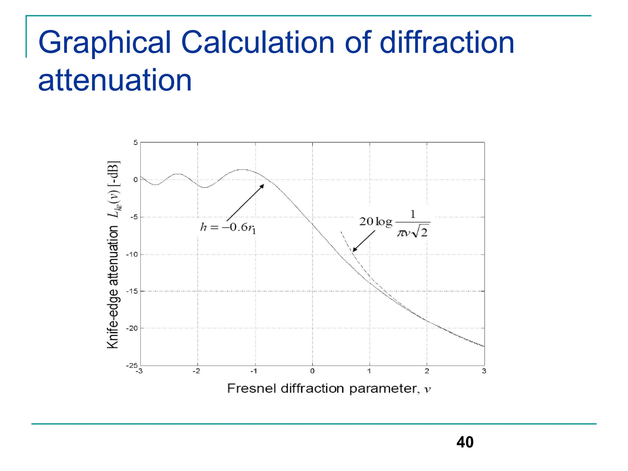
![Numerical solution
An approximate numerical solution for
equation
Can be found using set of equations given
below for different values of v
41
[0,1]
20 log(0.5 e- 0.95v)
[-1,0]
20 log(0.5-0.62v)
> 2.4
20 log(0.225/v)
[1, 2.4]
20 log(0.4-(0.1184-(0.38-0.1v)2)1/2)
-1
0
v
Gd(dB)](https://image.slidesharecdn.com/wcunit2-240913235922-2639a41d/75/wireless-communication-important-topics-379-2048.jpg)


![Scattering
Rayleigh criterion: used for testing surface roughness
A surface is considered smooth if its min to max protuberance (bumps)
h is less than critical height hc
hc = λ/8 sinΘi
Scattering path loss factor ρs is given by
ρs =exp[-8[(π*σh *sinΘi)/ λ] 2]
Where h is surface height and σh is standard deviation of surface
height about mean surface height.
For rough surface, the flat surface reflection coefficient is multiplied by
scattering loss factor ρs to account for diminished electric field
Reflected E-fields for h> hc for rough surface can be calculated as
Гrough= ρsГ
50](https://image.slidesharecdn.com/wcunit2-240913235922-2639a41d/75/wireless-communication-important-topics-388-2048.jpg)


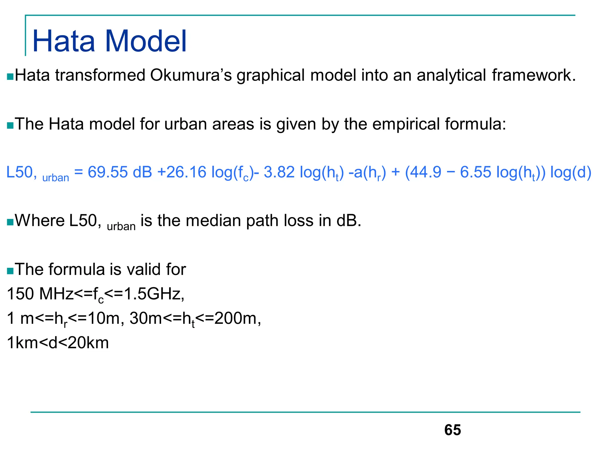
![Hata Model
The correction factor a(hr) for mobile antenna height hr for a small or
medium-sized city is given by:
a(hr) = (1.1 logfc − 0.7)hr − (1.56 log(fc) − 0.8) dB
For a large city it is given by
a(hr) = 8.29[log(1.54hr)]2 − 1.10 dB for fc <=300 MHz
3.20[log (11.75hr)]2 − 4.97 dB for fc >= 300 MHz
To obtain path loss for suburban area the standard Hata model is
modified as
L50 =L50(urban)-2[log(fc/28)]2-5.4
For rural areas
L50 =L50(urban)-4.78log(fc)2-18.33logfc -40.98
66](https://image.slidesharecdn.com/wcunit2-240913235922-2639a41d/75/wireless-communication-important-topics-404-2048.jpg)


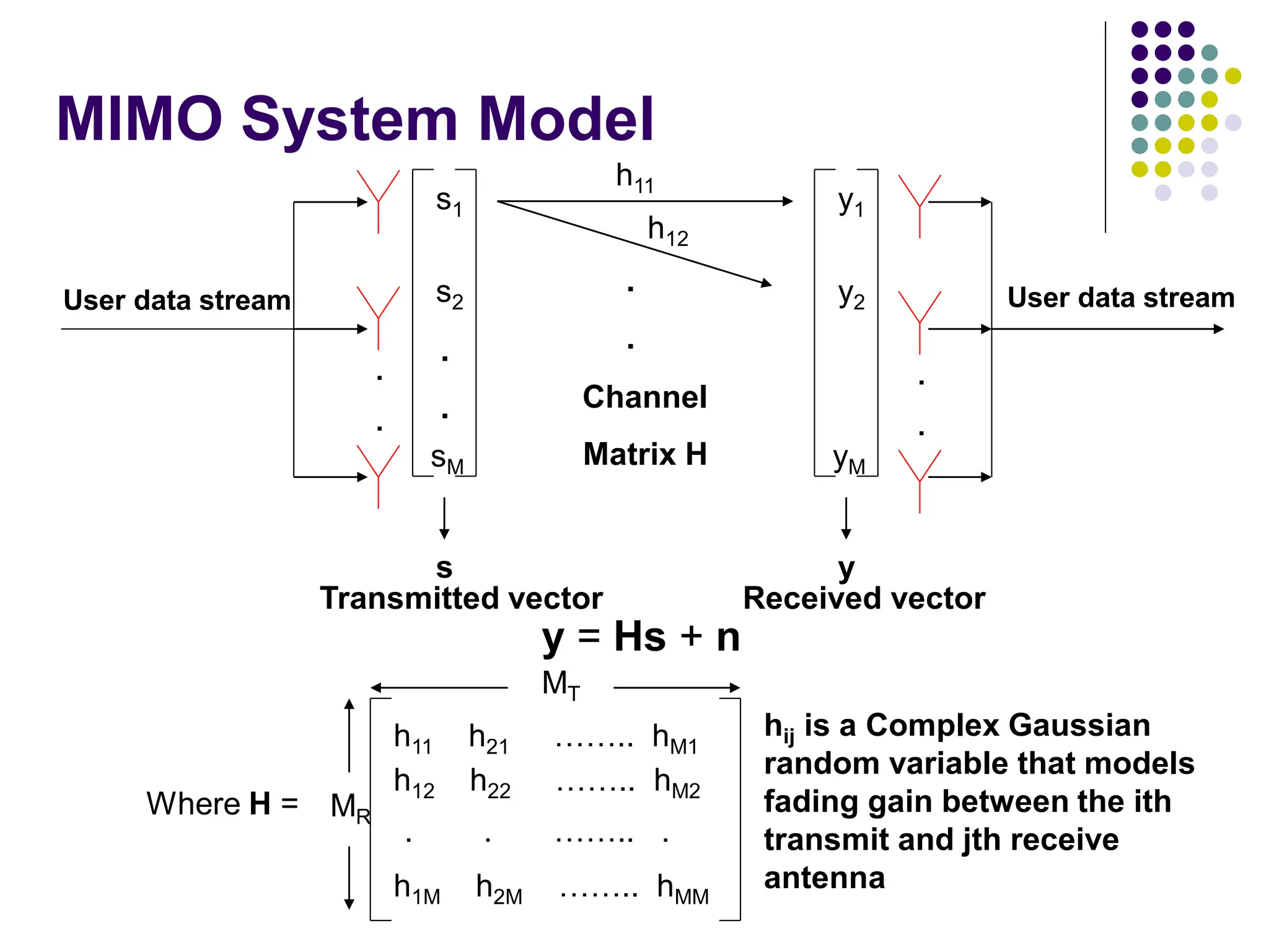
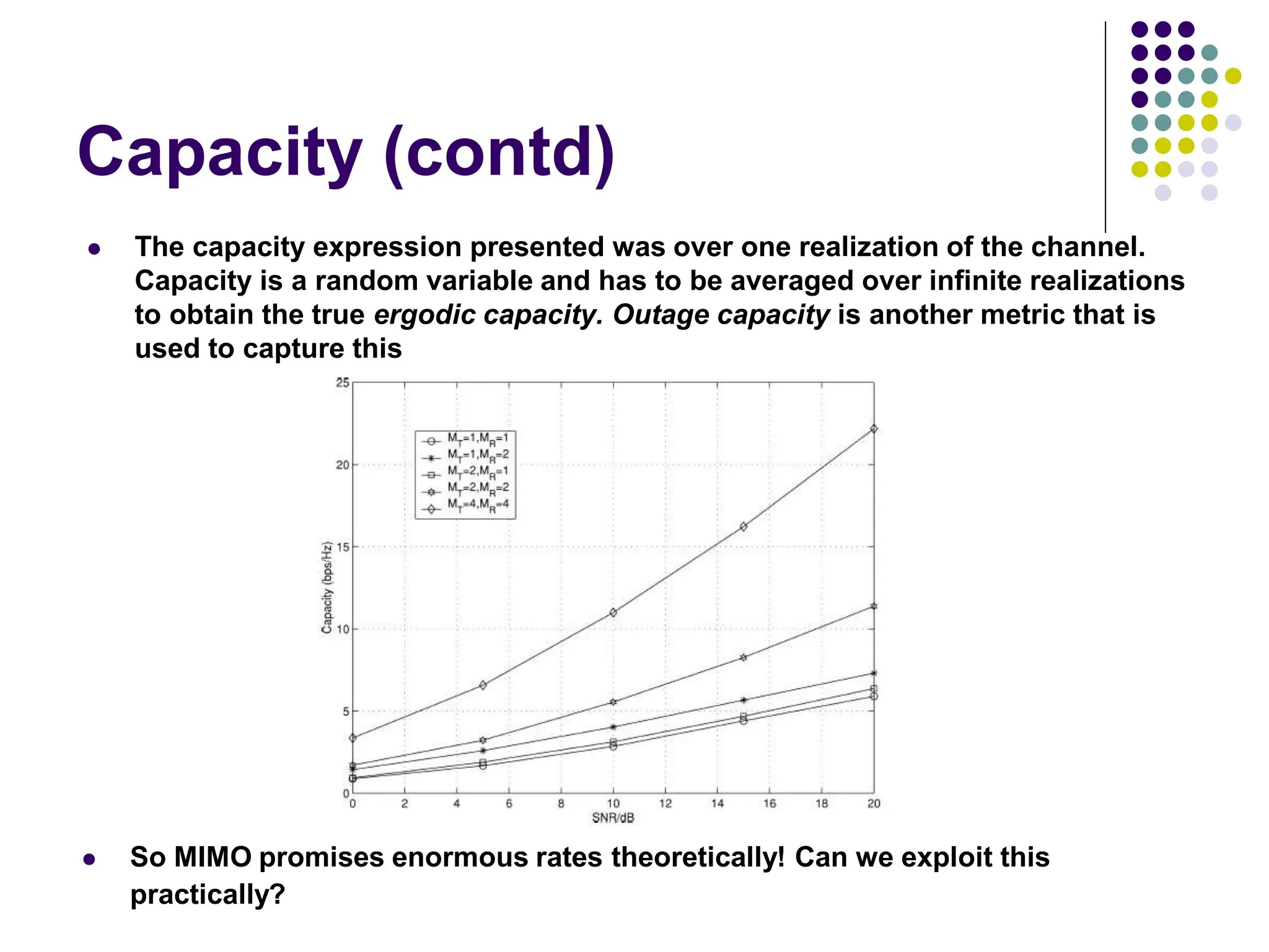
![Capacity of MIMO Channels
y = Hs + n
Let the transmitted vector s be a random vector to be very general and n is normalized
noise. Let the total transmitted power available per symbol period be P. Then,
C = log 2 (IM + HQHH) b/s/Hz
where Q = E{ssH} and trace(Q) < P according to our power constraint
Consider specific case when we have users transmitting at equal power over the channel
and the users are uncorrelated (no feedback available). Then,
CEP = log 2 [IM + (P/MT)HHH] b/s/Hz
Telatar showed that this is the optimal choice for blind transmission
Foschini and Telatar both demonstrated that as MT and MR grow,
CEP = min (MT,MR) log 2 (P/MT) + constant b/s/Hz
Note: When feedback is available, the Waterfilling solution is yields maximum capacity but converges to equal power capacity at
high SNRs](https://image.slidesharecdn.com/wcunit2-240913235922-2639a41d/75/wireless-communication-important-topics-459-2048.jpg)

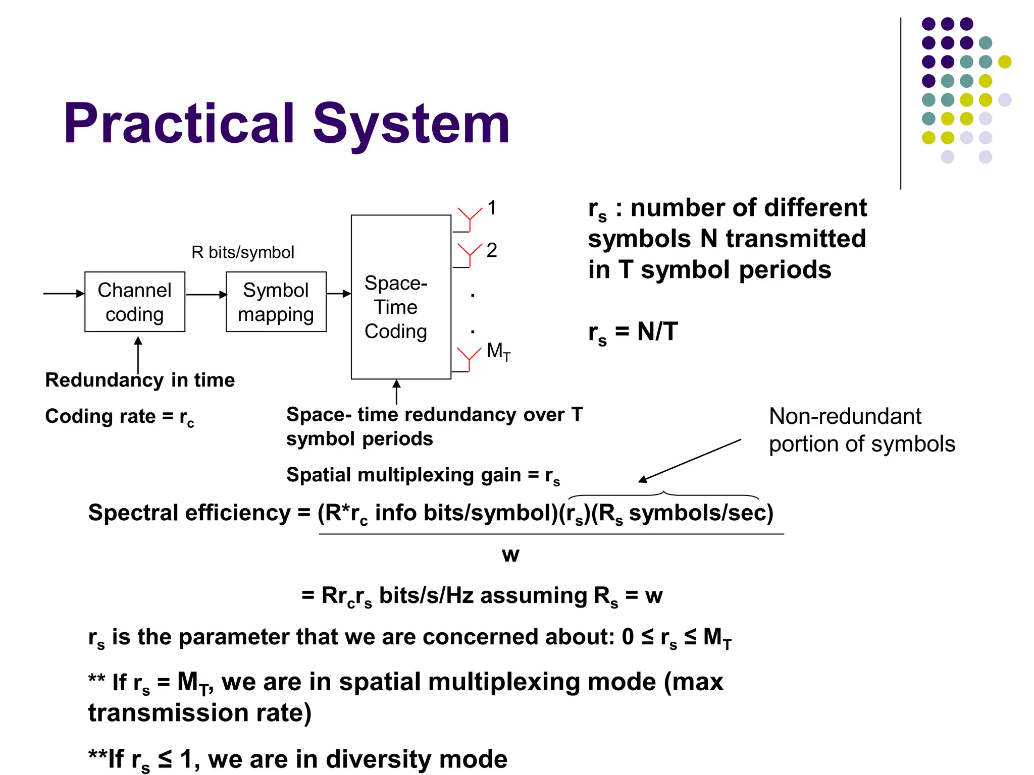
![Spatial Multiplexing
y = Hs + n y’ = Ds’ + n’ (through SVD on H)
where D is a diagonal matrix that contains the eigenvalues of HHH
Viewing the MIMO received vector in a different but equivalent
way,
CEP = log 2 [IM + (P/MT)DDH] = log 2 [1 + (P/MT)גi] b/s/Hz
Equivalent form tells us that an (MT,MR) MIMO channel opens up
m = min (MT,MR) independent SISO channels between the
transmitter and the receiver
So, intuitively, I can send a maximum of m different information
symbols over the channel at any given time
m
i 1](https://image.slidesharecdn.com/wcunit2-240913235922-2639a41d/75/wireless-communication-important-topics-463-2048.jpg)
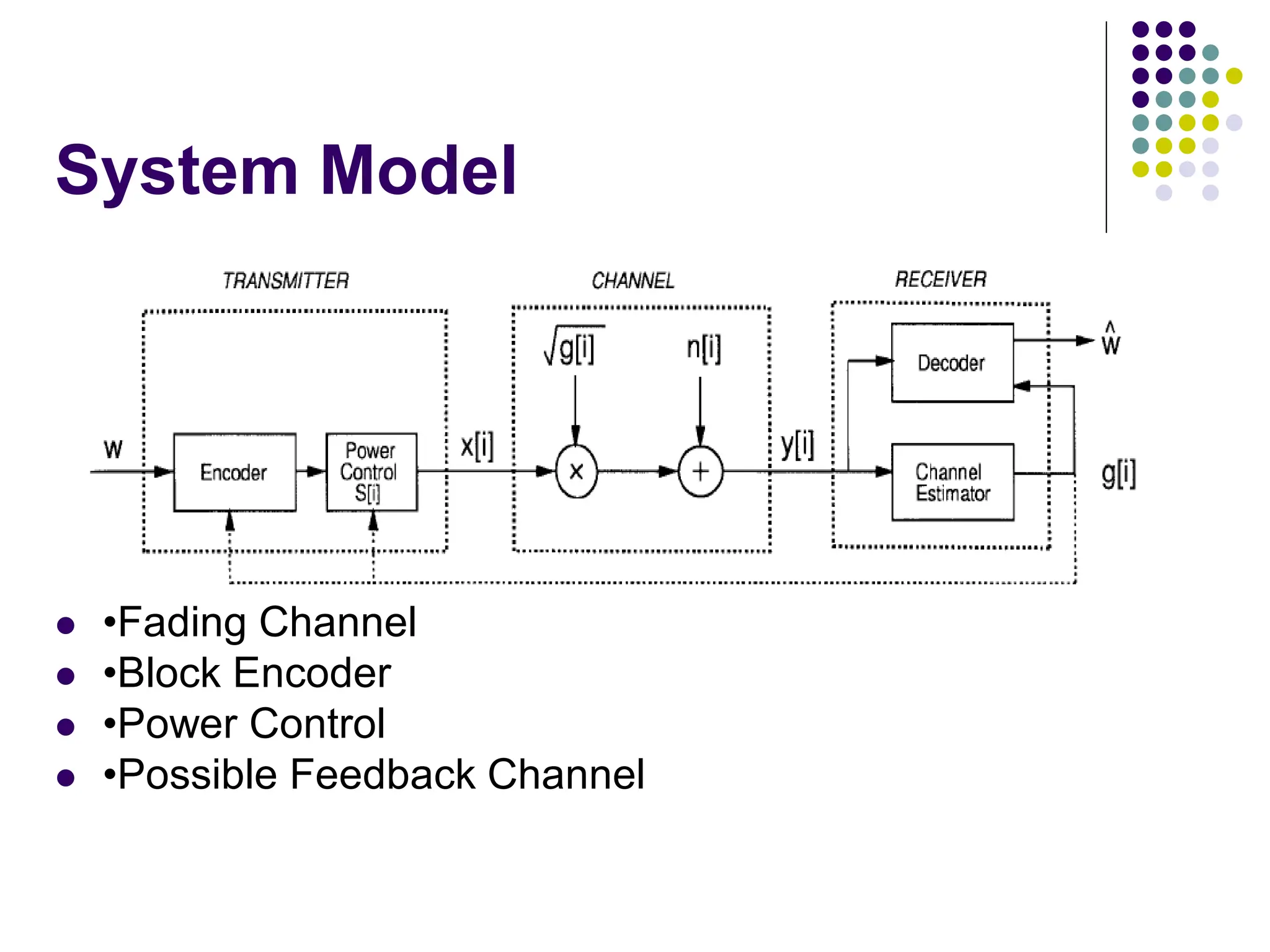
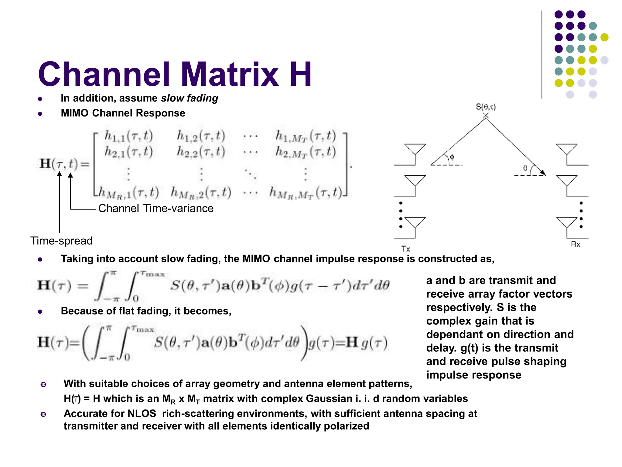
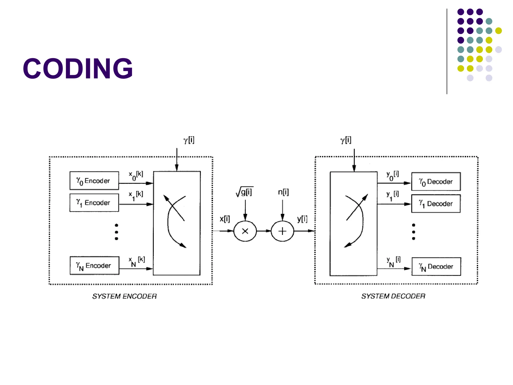
![System Model
The system model in figure 1 is a discrete-time channel with Stationary ergodic time-varying gain=
AWGN = n[i]
Channel power gain = g[i] is independent of the channel input and has an expected value of unity.
Average transmit signal power =S
Noise density = №
Received signal bandwidth =B
The instantaneous received signal-to-noise ratio (SNR),
S=(№B).
The system model, which sends an input message w from the
transmitter to the receiver.
The message is encoded into the codeword x, which is transmitted over the time-varying channel
as x[i] at time i.
The channel gain g[i] changes over the transmission of the codeword.
We assume perfect instantaneous channel estimation so that the channel power gain g[i] is known
to the receiver at time i.
We also consider the case when g[i] is known to both the receiver and transmitter at time i, as
might be obtained through an error-free delayless feedback path.
This allows the transmitter to adapt x[i] to the channel gain at time i, and is a reasonable model
for a slowly varying channel with channel estimation and transmitter feedback.](https://image.slidesharecdn.com/wcunit2-240913235922-2639a41d/75/wireless-communication-important-topics-477-2048.jpg)
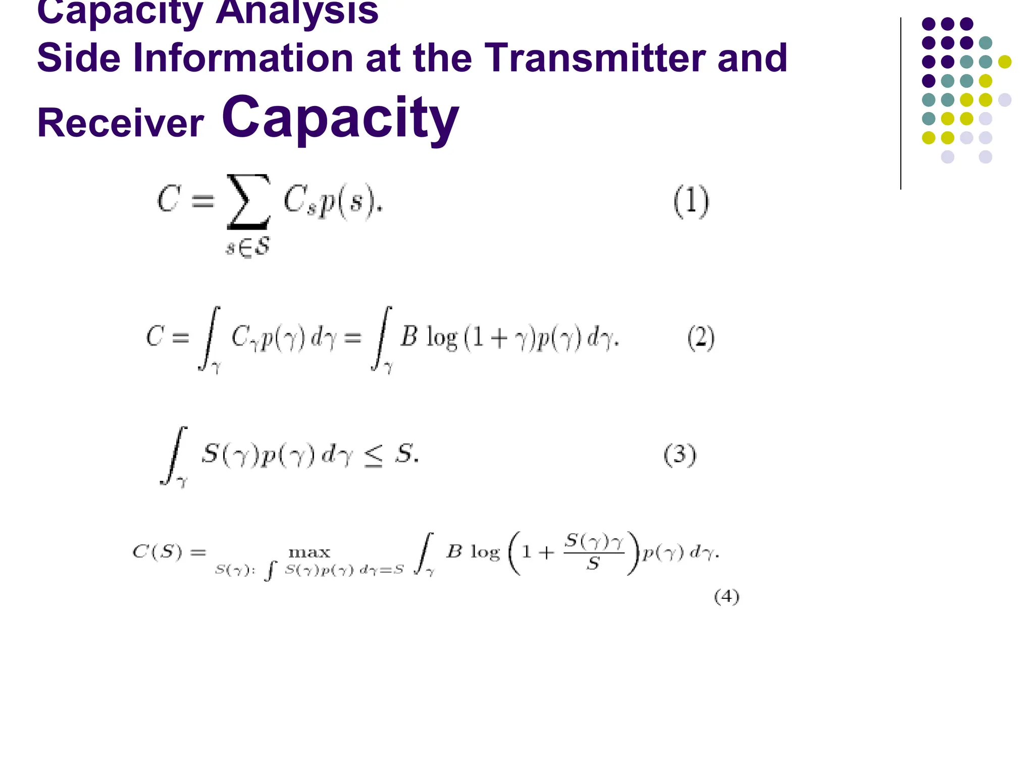
![Nonadaptive Technique
If g[i] is known at the decoder then by scaling, the fading
channel with power gain g[i] is equivalent to an AWGN
channel with noise power N0B/g[i].
If the transmit power is fixed at S and g[i] is i.i.d. then the
input distribution at time i which achieves capacity is an
i.i.d. Gaussian distribution with average power S.
The channel capacity with i.i.d. fading and receiver side
information only is given by:](https://image.slidesharecdn.com/wcunit2-240913235922-2639a41d/75/wireless-communication-important-topics-483-2048.jpg)