Testability Measures

1. 1
Contd...
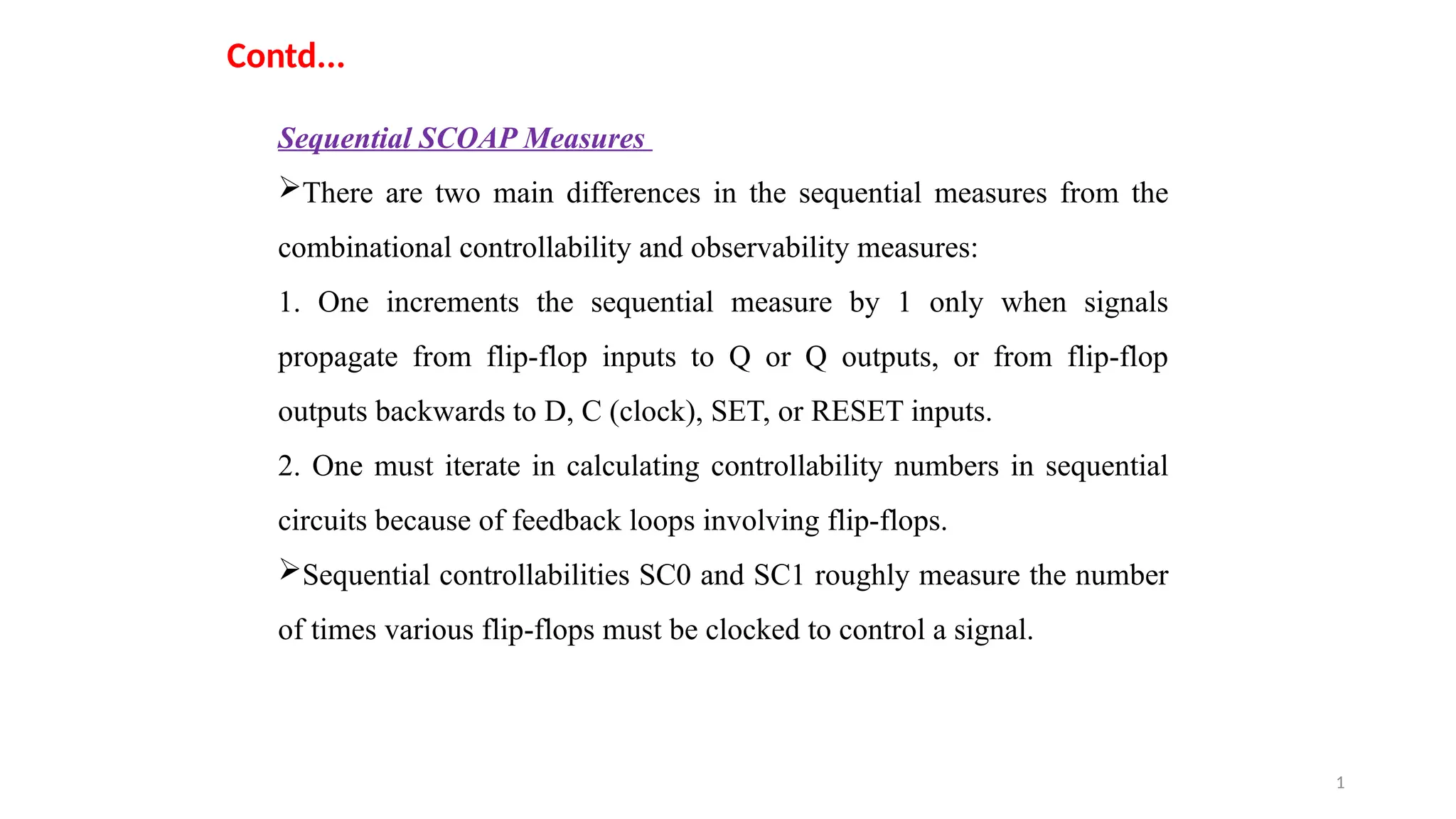
Sequential SCOAP Measures
There are two main differences in the sequential measures from the
combinational controllability and observability measures:
1. One increments the sequential measure by 1 only when signals
propagate from flip-flop inputs to Q or Q outputs, or from flip-flop
outputs backwards to D, C (clock), SET, or RESET inputs.
2. One must iterate in calculating controllability numbers in sequential
circuits because of feedback loops involving flip-flops.
Sequential controllabilities SC0 and SC1 roughly measure the number
of times various flip-flops must be clocked to control a signal.

2. 2
Contd...
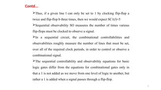
Thus, if a given line l can only be set to 1 by clocking flip-flop a
twice and flip-flop b three times, then we would expect SC1(l)=5
Sequential observability SO measures the number of times various
flip-flops must be clocked to observe a signal.
In a sequential circuit, the combinational controllabilities and
observabilities roughly measure the number of lines that must be set,
over all of the required clock periods, in order to control or observe a
combinational signal.
The sequential controllability and observability equations for basic
logic gates differ from the equations for combinational gates only in
that a 1 is not added as we move from one level of logic to another, but
rather a 1 is added when a signal passes through a flip-flop.

3. 3
Contd...
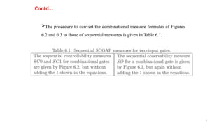
The procedure to convert the combinational measure formulas of Figures
6.2 and 6.3 to those of sequential measures is given in Table 6.1.

4. 4
Contd...
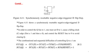
Figure 6.11 shows a synchronously resettable negative-edge-triggered D
flip-flop.
In order to control the Q line to 1, one must set D to 1, cause a falling clock
(C) edge (first a 1 and then a 0), and control the RESET line to 0 to avoid
clearing Q.
The combinational and sequential difficulties of controlling Q to a 1 are

5. 5
Contd...
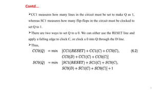
CC1 measures how many lines in the circuit must be set to make Q as 1,
whereas SC1 measures how many flip-flops in the circuit must be clocked to
set Q to 1.
There are two ways to set Q to a 0. We can either use the RESET line and
apply a falling edge to clock C, or clock a 0 into Q through the D line.
Thus,

6. 6
Contd...
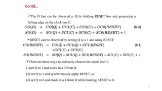
The D line can be observed at Q by holding RESET low and generating a
falling edge on the clock line C:
RESET can be observed by setting Q to a 1 and using RESET:
There are three ways to indirectly observe the clock line C:
(1)set Q to 1 and clock in a 0 from D,
(2) set Q to 1 and synchronously apply RESET, or
(3) set Q to 0 and clock in a 1 from D while holding RESET to 0.

7. 7
Contd...
Thus,

8. 8
Contd...
Algorithm 6.2 Compute combinational and sequential measures

9. 9
Contd...
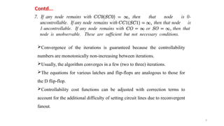
Convergence of the iterations is guaranteed because the controllability
numbers are monotonically non-increasing between iterations.
Usually, the algorithm converges in a few (two to three) iterations.
The equations for various latches and flip-flops are analogous to those for
the D flip-flop.
Controllability cost functions can be adjusted with correction terms to
account for the additional difficulty of setting circuit lines due to reconvergent
fanout.

10. 10
Contd...
The SCOAP measures can be enhanced to reflect this by adding in the term
fl -1 to every controllability calculation for CC0, CC1, SC0, and SC1, where
fl is the number of fanouts of a line l.
6.1.4 Sequential Circuit Example
On circuit lines in this example, CC0, CC1, and CO are shown as
(CC0,CC1)CO and SC0, SC1, and SO are shown as [SC0, SC1]SO below the
combinational measures.
The observabilities are always shown in bold to avoid confusion.
The forward level numbers for logic gates and flip-flops are shown circled
over the gates.
For backward level numbers during observability calculation, we just use
the forward level numbers in decreasing order from 5 down to 1.

11. 11
Contd...
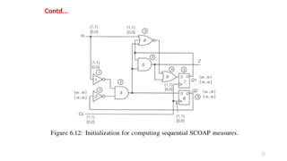
For level numbering flip-flops, we treat them like ordinary logic gates, and
ignore their feedback loops.
Figure 6.12 shows the initial measures for the example of Figure 6.4.
Signals R and CL, and all of their fanouts, are set to (CC0,CC1)=(1,1)and
[SC0,SC1]=[0,0]
All other nodes, particularly Q1 and Q2, are set to (CC0,CC1)=(,) and
[SC0,SC1]=[,]

12. 12
Contd...

13. 13
Contd...

14. 14
Contd...
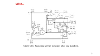
In Figure 6.13, we start the input to output computation of controllabilities.
Thus the output of INVERTER 1 is set to (CC0,CC1)=(2,2)and
[SC0,SC1]=[0,0] according to Figure 6.3 and Table 6.1. INVERTER 2 is
more interesting, because the feedback loop means that its measures must
remain at 
For AND gate 3, since 0 is a controlling value, we can determine CC0 and
SC0 measures of its output from Figure 6.3 and Table 6.1, as shown in Figure
6.13.
However, its CC1 and SC1 measures remain at A similar situation arises at
AND gate 5 in Figure 6.13.
ForNORgate4,CC0(4)=min(CC1(R),CC1(Q1),CC1(3))+1=min(1,,)+1=2

15. 15
Contd...
Similarly, SC0(4)=0.
An analogous situation occurs at OR gate 6.
At this point, 0-controllabilities are defined on both D inputs to the flip-
flops, but 1-controllabilities remain 
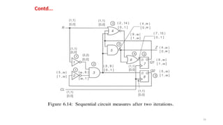
Figure 6.14 shows the situation after two iterations.
By Equations 6.2, CC0(7)=CC0(6)+CC1(CL)+CC0(CL)=7+1+1=9
The CC1, SC0, and SC1 measures for both flip-flops follow from
Equations 6.2 and 6.1.
Now, output controllabilities of INVERTER 2 change to (,6) and [,1]
This allows AND gate 3’s output CC1 measure to change to 9 and its
output SC1 measure to change to 1.

16. 16
Contd...

17. 17
Contd...
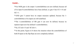
For NOR gate 4, the output 1-controllabilities are now defined, because all
of its input 0-controllabilities have been defined, so gate 4 has CC1=14 and
SC1=1.
AND gate 5 cannot have its output measures updated, because the 1-
controllabilities of its inputs are still undefined.
The 1-controllabilities of OR gate 6 can now be defined, because its
topmost input now has defined 1-controllabilities.
So, CC1(6)=15 and SC1(6)=1.
At this point, Figure 6.14 shows the situation where the controllabilities of
both D inputs to the flip-flops are now completely defined.

18. 18
Contd...
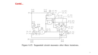
Figure 6.15 shows the situation after three iterations.
Equations 6.2 and 6.1 cause flip-flop 7s output controllabilities to
become (9,17) and [1,2].
Flip-flop 8’s controllabilities become (5,11) and [1,2]. INVERTER 2’s
output controllabilities become (12,6) and [2,1].
However, this causes no change in AND gate 3’s output controllabilities.
NOR gate 4’s CC1 stays at 14, and AND gate 5’s CC1 is now defined as
27 and its SC1 is now defined as 3.
The changes at gates 4 and 5 now cause no change at gate 6: CC1 stays
at 15.
 Figure 6.15 illustrates the situation at this point.

19. 19
Contd...

20. 20
Contd...

21. 21
Contd...

22. 22
Contd...
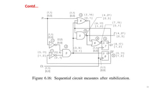
One more iteration results in the values shown in Figure 6.16.
We notice that all combinational and sequential controllabilities are
exactly the same as in Figure 6.15 after the third iteration.
Such stabilization always occurs in SCOAP.
The values in Figure 6.16 are the final controllabilities.
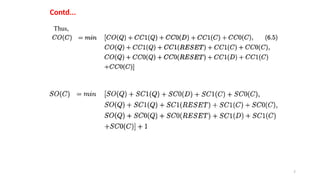
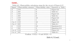
Rather than presenting the calculation of observabilities in running text,
we list in Table 6.2 all of the observabilities in their order of computation,
and give the equation or table that allows us to compute the observability.
The only difficult step is computing CO from line CL to 7 which is
CO=CO(Q)+CC1(CL)+CC0(CL)+CC0(D)+CC1(Q)=10+1+1+7+17=36 by
Equation 6.5.
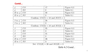
For the same line,SO=SO(Q)+SC1(CL)+SC0(CL)+SC0(D)+SC1(Q)+1
=1+0+0+0+2+1=4,also by Equation 6.5.

23. 23
Contd...
Table 6.2 Contd...

24. 24
Contd...
Table 6.2 Contd...

25. 25
Contd...
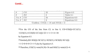
For the CO of the line from CL to line 8, CO=CO(Q)+CC1(CL)
+CC0(CL)+CC0(D)+CC1(Q)=22+1+1+3+11=38
by Equation 6.5.
Similarly,SO=SO(Q)+SC1(CL)+SC0(CL)+SC0(D)+SC1(Q)
+1=2+0+0+0+2+1=5 also by Equation 6.5.
Therefore, CO(CL)=min(36,38)=36 and SO(CL)=min(4,5)=4.

26. 26
Contd...
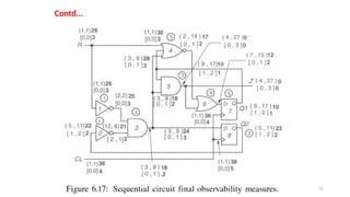
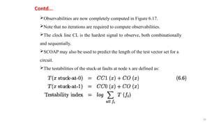
Observabilities are now completely computed in Figure 6.17.
Note that no iterations are required to compute observabilities.
The clock line CL is the hardest signal to observe, both combinationally
and sequentially.
SCOAP may also be used to predict the length of the test vector set for a
circuit.
The testabilities of the stuck-at faults at node x are defined as:

27. 27
Contd...
In order to detect a fault at x, one must set x to the opposite value from the
fault and observe x at a PO.
Figure 6.18 shows a linear relationship between the number of vectors
needed for 90% fault coverage and the Testability index for a number of
circuits.