Deep learning

1. Chap 5
Machine Learning Basics
Dr.Anand Kumar M

5. Introduction
• Machine Learning
– Form of applied statistics with extensive use of
computers to estimate complicated functions
• Two categories of machine learning
– Supervised learning and unsupervised learning
• Most machine learning algorithms based on
stochastic gradient descent optimization

6. 1 Learning Algorithms
• A machine learning algorithm learns from data
• A computer program learns from
– experience E
– with respect to some class of tasks T
– and performance measure P
– if it’s performance P on tasks T improves with
experience E

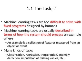
7. 1.1 The Task, T
• Machine learning tasks are too difficult to solve with
fixed programs designed by humans
• Machine learning tasks are usually described in
terms of how the system should process an example
where
– An example is a collection of features measured from an
object or event
• Many kinds of tasks
– Classification, regression, transcription, anomaly
detection, imputation of missing values, etc.

8. 1.2 The Performance Measure, P
• Performance P is usually specific to the Task T
• For classification tasks, P is usually accuracy
– The proportion of examples correctly classified
– Here we are interested in the accuracy on data not seen
before – a test set

9. 1.3 The Experience, E
• Most learning algorithms are allowed to experience
an entire dataset
• Unsupervised learning algorithms
– Learn useful structural properties of the dataset
• Supervised learning algorithms
– Experience a dataset containing features with each
example associated with a label or target
• For example, target provided by a teacher
• Blur between supervised and unsupervised

10. 2 Capacity, Overfitting
and Underfitting
• The central challenge in machine learning is to
perform well on new, previously unseen inputs, and
not just on the training inputs
• We want the generalization error (test error) to be
low as well as the training error
• This is what separates machine learning from
optimization

11. 2 Capacity, Overfitting
and Underfitting
• How can we affect performance on the test set
when we get to observe only the training set?
• Statistical learning theory provides answers
• We assume train and test sets are generated
independent and identically distributed – i.i.d.
• Thus, expected train and test errors are equal

12. 2 Capacity, Overfitting
and Underfitting
• Because the model is developed from the training
set the expected test error is usually greater than
the expected training error
• Factors determining machine performance are
– Make the training error small
– Make the gap between train and test error small
• These two factors correspond to the two challenges
in machine learning
– Underfitting and overfitting

13. 2 Capacity, Overfitting
and Underfitting
• Underfitting and overfitting can be controlled
somewhat by altering the model’s capacity
– Capacity = model’s ability to fit variety of functions
• Low capacity models struggle to fit the training data
• High capacity models can overfit the training data
• One way to control the capacity of a model is by
choosing its hypothesis space
– For example, simple linear vs quadratic regression

14. Underfitting and Overfitting in Polynomial
Estimation
x0
y
Underfitting Appropriate capacity
Overfitting
Figure
(Goodfellow 2016)
x0
y
x0
y

15. 2 Capacity, Overfitting
and Underfitting
• Model capacity can be changed in many ways –
above we changed the number of parameters
• We can also change the family of functions –called
the model’s representational capacity
• Statistical learning theory provides various means of
quantifying model capacity
– The most well-known is the Vapnik-Chervonenkis
dimension
– Old non-statistical Occam’s razor method takes simplest
of competing hypotheses

16. 2 Capacity, Overfitting
and Underfitting
• While simpler functions are more likely to
generalize (have a small gap between training and
test error) we still want low training error
• Training error usually decreases until it asymptotes
to the minimum possible error
• Generalization error usually has a U-shaped curve
as a function of model capacity

17. Generalization and Capacity
0 Optimal Capacity
Capacity
Error
Underfitting zone Overfitting
zone
Generalization gap
Training error
Generalization error
Figure
(Goodfellow 2016)

18. 2 Capacity, Overfitting
and Underfitting
• Non-parametric models can reach arbitrarily high
capacities
• For example, the complexity of the nearest
neighbor algorithm is a function of the training set
size
• Training and generalization error vary as the size of
the training set varies
– Test error decreases with increased training set size

19. (Goodfellow 2016)
Training Set Size
100
101
102
103
Number of training
examples
104
105
0.
0
3.5
3.0
2.5
2.0
1.
5
1.0
0.5
Error
(MSE)
Bayes error
Train (quadratic) Test
(quadratic)
Test (optimal capacity)
Train (optimal
capacity)
100
101
102
103
Number of training
104
105
20
15
10
5
0
Optimal
capacity
(polynomial
degree)
Figure 5.4