The document discusses a finite element analysis of a double-cantilever beam (DCB) specimen with delamination, utilizing a 3D elasticity model to solve for the energy release rate (G_i) in two distinct laminate configurations. It confirms that the approximation error is less than 1% and highlights the differences between results from various material layups, noting that the laminate stack exhibits a lower and slower rise in energy release rate compared to other configurations. Additionally, the document provides insight into the effects of meshing and boundary conditions on the accuracy of results in both 3D and 2D problem formulations.

1. Problem 4-5: DCB Specimen – Computation of ERR
Yichen Sun 446230
Consider the double-cantilever beam (DCB) specimen shown in Figure below with a
delamination of length “a”. The material is 24-ply T300 unidirectional graphite/epoxy
laminate with a layup [0]24 and the following properties:
EL = 139.4 GPa, ET=10.16 GPa, νLT = 0.30, νTT = 0.436, GLT = 4.6 GPa and GTT =
3.45 GPa
(a) Given B = 25.0 mm, 2h = 3.0 mm, 2L = 150 mm, a = 30 mm, δ = 2.0 mm, find the
distribution of GI
(b) Compare the results with a 2D plane-strain solution obtained using the finite
element method.
along the delamination front by solving a 3D problem of elasticity
using the finite element method.
(c) Repeat case (a) for the 24-ply T300 laminate with following layup:
[0/90/0/45/-45/0/45/-45/0/45/-45/0]S.
In all cases show evidence that the error of approximation is small (<1%) and
comment on the difference in results among all three cases. Are there significant
differences in G I for cases (a) and (c) even though the delamination is located
between two 0 deg. plies in both?
【Solution and Analysis】
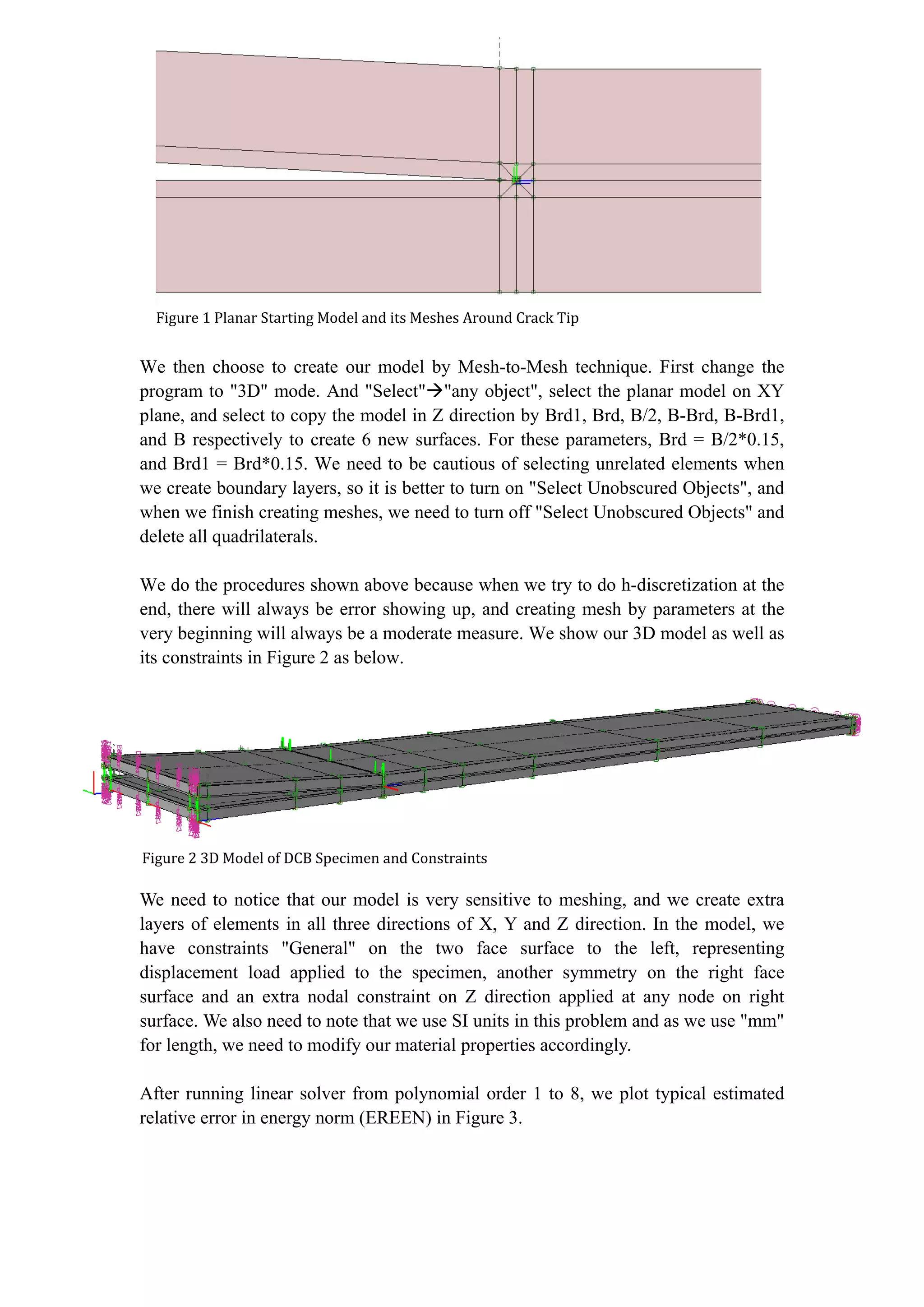
We first create a planar model of the front surface of the DCB specimen, and the part
near crack tip is shown in Figure 1. This planar model is created in the same fashion
as what we did in Problem 4-4 Case 3, in which we use a parameter "displacement" to
create a layer of overlapping mesh around the crack tip. When we set "displacement"
not equal to 0, the crack opens; and the crack closes when we set "displacement" 0.

2. We then choose to create our model by Mesh-to-Mesh technique. First change the
program to "3D" mode. And "Select""any object", select the planar model on XY
plane, and select to copy the model in Z direction by Brd1, Brd, B/2, B-Brd, B-Brd1,
and B respectively to create 6 new surfaces. For these parameters, Brd = B/2*0.15,
and Brd1 = Brd*0.15. We need to be cautious of selecting unrelated elements when
we create boundary layers, so it is better to turn on "Select Unobscured Objects", and
when we finish creating meshes, we need to turn off "Select Unobscured Objects" and
delete all quadrilaterals.
We do the procedures shown above because when we try to do h-discretization at the
end, there will always be error showing up, and creating mesh by parameters at the
very beginning will always be a moderate measure. We show our 3D model as well as
its constraints in Figure 2 as below.
We need to notice that our model is very sensitive to meshing, and we create extra
layers of elements in all three directions of X, Y and Z direction. In the model, we
have constraints "General" on the two face surface to the left, representing
displacement load applied to the specimen, another symmetry on the right face
surface and an extra nodal constraint on Z direction applied at any node on right
surface. We also need to note that we use SI units in this problem and as we use "mm"
for length, we need to modify our material properties accordingly.
After running linear solver from polynomial order 1 to 8, we plot typical estimated
relative error in energy norm (EREEN) in Figure 3.
Figure 1 Planar Starting Model and its Meshes Around Crack Tip
Figure 2 3D Model of DCB Specimen and Constraints

3. We see from Figure 3 that global error is reduced to 0.81% when p=8, and this global
error is pretty acceptable in the existence of a crack.
We then go to "Points" tab and choose to plot function J1 at crack front with a
integration radius of 6e-2, which is just outside the inner cube. In our 3D elasticity
problem, energy release rate GI is equivalent to J1
p
and we plot our results in run p=6,
7 and 8 in Figure 4 as below.
Figure 3 Typical Estimated Relative Error in Energy Norm
Figure 4 Results of J1
P
at Crack Front in Run P=6, 7 and 8

4. We could see from Figure 4 that results of J1
P
nearly overlap with each other,
indicating a low discretization error, and the J-integral rise quickly from around 0.14
Pa*m near both surfaces to around 0.31 Pa*m in the middle of the specimen.
We then plot in Figure 5 the value of J-integral at a point on the crack tip against DOF,
and we see the result converges to within 0.08% of the exact value, which also shows
pretty good convergence and low discretization error of J1.
We then try to obtain a result with a 2D plane-strain solution obtained using the finite
element method. In this case, we restrict our 3D model used with two symmetry
constraints on both front and back surface. This is because, a plane strain is the limit
case where the thickness goes to infinity, and our two symmetries on both faces
would accomplish this. We perform the same analysis as we did in case 1.
We go to "Points" tab and choose to plot function J1 at crack front with an integration
radius of 6e-2, which is just outside the inner cube, and "# of points"=10. We then plot
our results of J1
P
in run p=6, 7 and 8 in Figure 6 as below.
Figure 5 Convergence of J-Integral
Figure 6 Results of J1
P
at Crack Front in Run P=6, 7 and 8, 2D Case

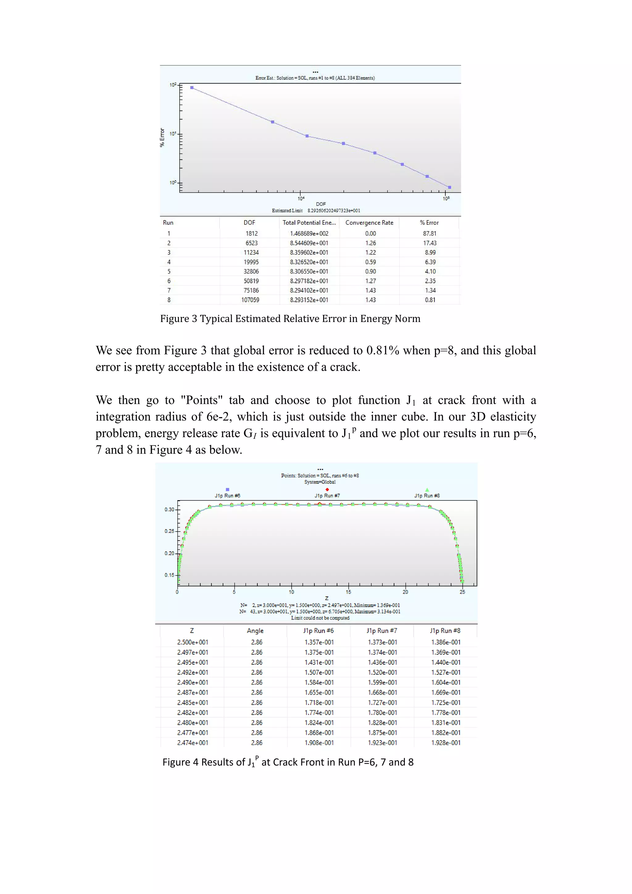
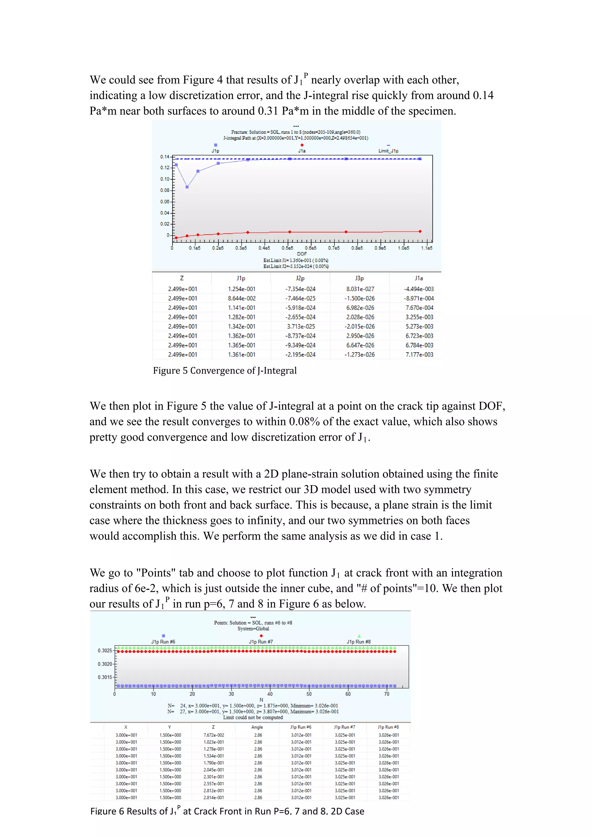
5. We see our J1
p
almost remains unchanged throughout thickness, with constant value
of 0.3025, and the convergence of results is also excellent as J1
p
in the last three runs
differ by no more than 0.5%..
At last, we repeat case (a) for the 24-ply T300 laminate with following layup:
[0/90/0/45/-45/0/45/-45/0/45/-45/0]S.
We first go to "Edit", "Laminate Info" and enters our record as shown in Figure 7
below. We then go to "Material", "assign" tab, choose our inverted coordinate system,
upper and lower face surfaces, "laminate-stack", "inverted" and select the laminate
material we just created. Note that inner most layer has a thickness of h/12 and in
laminate info, we choose number of layers 11 and assign all values as indicated in
Figure 7. And another illustration of laminate-stacked model is shown in Figure 8.
Figure 7 Laminate Properties and Laminate-Stacked Model
Figure 8 Laminate-Stacked Model with Representation of Layers

6. We just assign 11 piles of laminate stack to upper surface and lower surface
respectively. And we then run linear solver to check results of J1
P
as is shown in
Figure 9.
We see that the results of J1
P
nearly overlap with each for Run P=6, 7 and 8,
indicating a low discretization error, and the J-integral rises quickly from around
0.01584 Pa*m near both surfaces to around 0.2353 Pa*m in the middle of the
specimen. We could see that J1 distribution along crack edge has a similar distribution
than model 1 but rises less rapidly from both surfaces and is a little less in value than
that in our model 1.
Figure 9 Results of J1
P at Crack Front in Run P=6, 7 and 8，Laminate Stacked Model
Figure 10 Convergence of J-Integral at Z=8.013 along Crack Tip

7. We then plot in Figure 10 the value of J-integral at a point Z=8.013 on the crack tip
against DOF, and we see the result converges to within 0.29% of the exact value,
which also shows pretty good convergence and low discretization error of J1.
We are likely to conclude that energy release rate is higher in the middle of the
specimen and lower in the laminate stacked models, indicating harder to open up
crack near edges and in laminate stacked model.