Pitfalls in Relational-Database designs Concept of normalization, Function Dependencies First Normal Form, 2NF, 3NF, BCNF.

1. DATABASE
MANAGEMENT
SYSTEMS
Couse code:CSC403
Prof. Juhi Janjua

2. Module 3:
Relational Model
and relational
Algebra
• Introduction to the Relational Model
• Relational schema and concept of keys.
• Mapping the ER and EER Model to the Relational
Model
• Relational Algebra-operators
• Relational Algebra Queries.

3. Introduction to Relational Model
• Relational Model was proposed by E.F. Codd to model data
in the form of relations or tables.
• After designing the conceptual model of Database using ER
diagram, we need to convert the conceptual model in the
relational model which can be implemented using any
RDBMS languages like Oracle SQL, MySQL etc.
• So, we will see what Relational Model is.

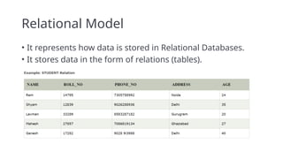
4. Relational Model
• It represents how data is stored in Relational Databases.
• It stores data in the form of relations (tables).

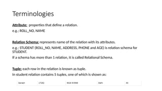
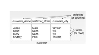
5. Terminologies
Attribute: properties that define a relation.
e.g.; ROLL_NO, NAME
Relation Schema: represents name of the relation with its attributes.
e.g.; STUDENT (ROLL_NO, NAME, ADDRESS, PHONE and AGE) is relation schema for
STUDENT.
If a schema has more than 1 relation, it is called Relational Schema.
Tuple: each row in the relation is known as tuple.
In student relation contains 5 tuples, one of which is shown as:

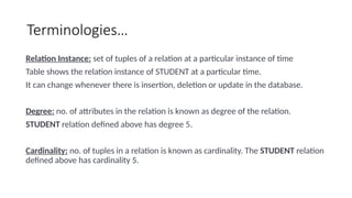
7. Terminologies…
Relation Instance: set of tuples of a relation at a particular instance of time
Table shows the relation instance of STUDENT at a particular time.
It can change whenever there is insertion, deletion or update in the database.
Degree: no. of attributes in the relation is known as degree of the relation.
STUDENT relation defined above has degree 5.
Cardinality: no. of tuples in a relation is known as cardinality. The STUDENT relation
defined above has cardinality 5.

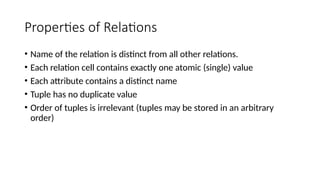
8. Properties of Relations
• Name of the relation is distinct from all other relations.
• Each relation cell contains exactly one atomic (single) value
• Each attribute contains a distinct name
• Tuple has no duplicate value
• Order of tuples is irrelevant (tuples may be stored in an arbitrary
order)

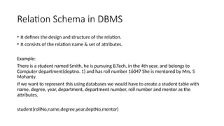
9. Relation Schema in DBMS
• It defines the design and structure of the relation.
• It consists of the relation name & set of attributes.
Example:
There is a student named Smith, he is pursuing B.Tech, in the 4th year, and belongs to
Computer department(deptno. 1) and has roll number 16047 She is mentored by Mrs. S
Mohanty.
If we want to represent this using databases we would have to create a student table with
name, degree, year, department, department number, roll number and mentor as the
attributes.
student(rollNo,name,degree,year,deptNo,mentor)

10. Relation schema…
This and other departments can be represented by the department table, having
department ID, name and hod as attributes.
department(deptID,name,hod)
The course that a student has selected has a courseid, course name, credit and department
number.
course(courseId,cname,credits,deptNo)
The professor would have an employee Id, name, department no. and phone number.
professor(empId,name,deptNo,phoneNo)

11. Relation schema…
We can have another table named enrollment (relationship between course &
student), which has roll no, courseId, semester, year and grade as the attributes.
enrollment(rollNo,courseId,sem,year,grade)
Teaching (relationship between professor & course) can be another table, having
employee id, course id, semester, year and classroom as attributes
teaching(empId,courseId,sem,year,classroom)
And so on…
Relations between them is represented through arrows

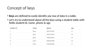
12. Concept of keys
• Keys are defined to easily identify any row of data in a table.
• Let's try to understand about all the keys using a student table with
fields student-id, name, phone & age

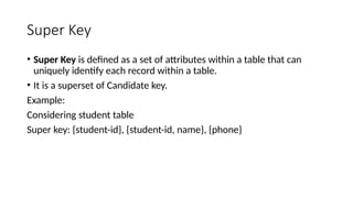
13. Super Key
• Super Key is defined as a set of attributes within a table that can
uniquely identify each record within a table.
• It is a superset of Candidate key.
Example:
Considering student table
Super key: {student-id}, {student-id, name}, {phone}

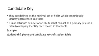
14. Candidate Key
• They are defined as the minimal set of fields which can uniquely
identify each record in a table.
• It is an attribute or a set of attributes that can act as a primary Key for a
table to uniquely identify each record in that table.
Example:
student-id & phone are candidate keys of student table

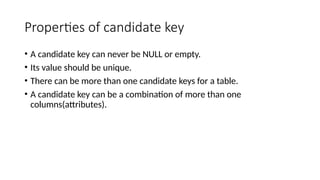
15. Properties of candidate key
• A candidate key can never be NULL or empty.
• Its value should be unique.
• There can be more than one candidate keys for a table.
• A candidate key can be a combination of more than one
columns(attributes).

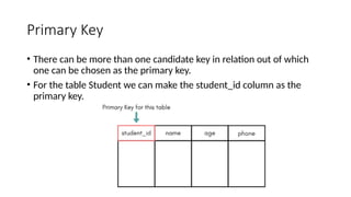
16. Primary Key
• There can be more than one candidate key in relation out of which
one can be chosen as the primary key.
• For the table Student we can make the student_id column as the
primary key.

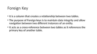
17. Foreign Key
• It is a column that creates a relationship between two tables.
• The purpose of Foreign keys is to maintain data integrity and allow
navigation between two different instances of an entity.
• It acts as a cross-reference between two tables as it references the
primary key of another table.

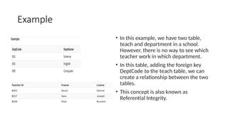
18. Example
• In this example, we have two table,
teach and department in a school.
However, there is no way to see which
teacher work in which department.
• In this table, adding the foreign key
DeptCode to the teach table, we can
create a relationship between the two
tables.
• This concept is also known as
Referential Integrity.

19. Mapping the ER and EER Model to the Relational Model

20. 20
Steps for mapping
• ER-to-Relational Mapping Algorithm
Step 1: Mapping of Regular Entity Types
Step 2: Mapping of Weak Entity Types
Step 3: Mapping of Binary 1:1 Relation Types
Step 4: Mapping of Binary 1:N Relationship Types.
Step 5: Mapping of Binary M:N Relationship Types.
Step 6: Mapping of Multivalued attributes.
Step 7: Mapping of N-ary Relationship Types.
• Mapping EER Model Constructs to Relations
Step 8: Options for Mapping Specialization or Generalization.
Step 9: Mapping of Union Types (Categories).

21. 21
Step 1: Mapping of Regular Entity Types.
• For each regular (strong) entity type E in the ER schema, create a
relation R that includes all the simple attributes of E.
• Choose one of the key attributes of E as the primary key for R. If the
chosen key of E is composite, the set of simple attributes that form it
will together form the primary key of R.

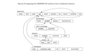
22. Step 1
Example: We create the relations
EMPLOYEE, DEPARTMENT, and
PROJECT in the relational schema
corresponding to the regular
entities in the ER diagram. SSN,
DNUMBER, and PNUMBER are the
primary keys for the relations
EMPLOYEE, DEPARTMENT, and
PROJECT as shown.

23. 23
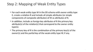
Step 2: Mapping of Weak Entity Types
• For each weak entity type W in the ER schema with owner entity type
E, create a relation R and include all simple attributes (or simple
components of composite attributes) of W as attributes of R.
• In addition, include as foreign key attributes of R the primary key
attribute(s) of the relation(s) that correspond to the owner entity
type(s).
• The primary key of R is the combination of the primary key(s) of the
owner(s) and the partial key of the weak entity type W, if any.

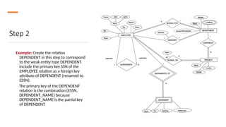
24. Step 2
Example: Create the relation
DEPENDENT in this step to correspond
to the weak entity type DEPENDENT.
Include the primary key SSN of the
EMPLOYEE relation as a foreign key
attribute of DEPENDENT (renamed to
ESSN).
The primary key of the DEPENDENT
relation is the combination {ESSN,
DEPENDENT_NAME} because
DEPENDENT_NAME is the partial key
of DEPENDENT.

25. 25
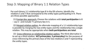
Step 3: Mapping of Binary 1:1 Relation Types
For each binary 1:1 relationship type R in the ER schema, identify the
relations S and T that correspond to the entity types participating in R. There
are three possible approaches:
(1) Foreign Key approach: Choose the relations with total participation in R
– say S-- and include T’s primary key in S.
(2) Merged relation option: An alternate mapping of a 1:1 relationship type
is possible by merging the two entity types and the relationship into a single
relation. This may be appropriate when both participations are total.
(3) Cross-reference or relationship relation option: The third alternative is
to set up a third relation W(T.primarykey, S.primaryKey) for the purpose of
cross-referencing the primary keys of the two relations S and T representing
the entity types.

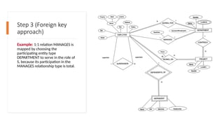
26. Step 3 (Foreign key
approach)
Example: 1:1 relation MANAGES is
mapped by choosing the
participating entity type
DEPARTMENT to serve in the role of
S, because its participation in the
MANAGES relationship type is total.

27. 27
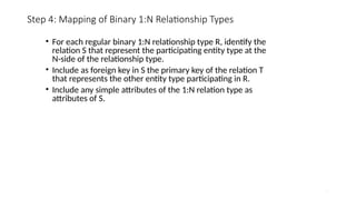
Step 4: Mapping of Binary 1:N Relationship Types
• For each regular binary 1:N relationship type R, identify the
relation S that represent the participating entity type at the
N-side of the relationship type.
• Include as foreign key in S the primary key of the relation T
that represents the other entity type participating in R.
• Include any simple attributes of the 1:N relation type as
attributes of S.

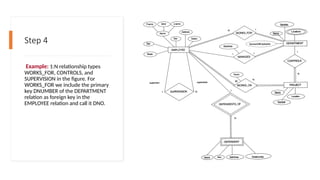
28. Step 4
Example: 1:N relationship types
WORKS_FOR, CONTROLS, and
SUPERVISION in the figure. For
WORKS_FOR we include the primary
key DNUMBER of the DEPARTMENT
relation as foreign key in the
EMPLOYEE relation and call it DNO.

29. 29
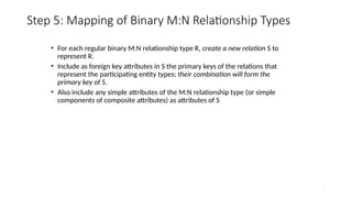
Step 5: Mapping of Binary M:N Relationship Types
• For each regular binary M:N relationship type R, create a new relation S to
represent R.
• Include as foreign key attributes in S the primary keys of the relations that
represent the participating entity types; their combination will form the
primary key of S.
• Also include any simple attributes of the M:N relationship type (or simple
components of composite attributes) as attributes of S

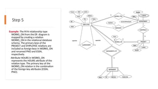
30. Step 5
Example: The M:N relationship type
WORKS_ON from the ER diagram is
mapped by creating a relation
WORKS_ON in the relational database
schema. The primary keys of the
PROJECT and EMPLOYEE relations are
included as foreign keys in WORKS_ON
and renamed PNO and ESSN,
respectively.
Attribute HOURS in WORKS_ON
represents the HOURS attribute of the
relation type. The primary key of the
WORKS_ON relation is the combination
of the foreign key attributes {ESSN,
PNO}.

31. 31
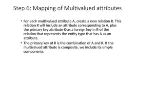
Step 6: Mapping of Multivalued attributes
• For each multivalued attribute A, create a new relation R. This
relation R will include an attribute corresponding to A, plus
the primary key attribute K-as a foreign key in R-of the
relation that represents the entity type that has A as an
attribute.
• The primary key of R is the combination of A and K. If the
multivalued attribute is composite, we include its simple
components.

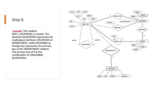
32. Step 6
Example: The relation
DEPT_LOCATIONS is created. The
attribute DLOCATION represents the
multivalued attribute LOCATIONS of
DEPARTMENT, while DNUMBER-as
foreign key-represents the primary
key of the DEPARTMENT relation.
The primary key of R is the
combination of {DNUMBER,
DLOCATION}.

33. 33
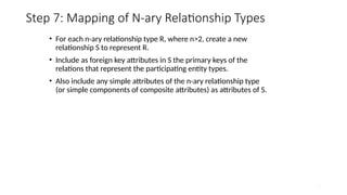
Step 7: Mapping of N-ary Relationship Types
• For each n-ary relationship type R, where n>2, create a new
relationship S to represent R.
• Include as foreign key attributes in S the primary keys of the
relations that represent the participating entity types.
• Also include any simple attributes of the n-ary relationship type
(or simple components of composite attributes) as attributes of S.

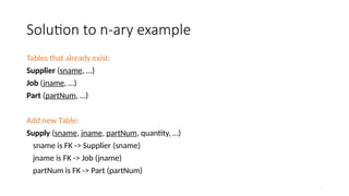
34. Step 7
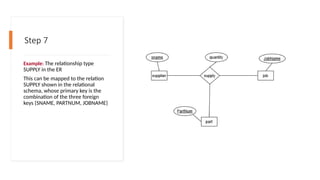
Example: The relationship type
SUPPLY in the ER
This can be mapped to the relation
SUPPLY shown in the relational
schema, whose primary key is the
combination of the three foreign
keys {SNAME, PARTNUM, JOBNAME}

35. 35
Solution to n-ary example
Tables that already exist:
Supplier (sname, …)
Job (jname, …)
Part (partNum, …)
Add new Table:
Supply (sname, jname, partNum, quantity, …)
sname is FK -> Supplier (sname)
jname is FK -> Job (jname)
partNum is FK -> Part (partNum)

36. 36
Result of mapping the COMPANY ER schema into a relational schema.

37. Summary of mapping constructs &
constraints

38. 38
Mapping EER Model Constructs to
Relations
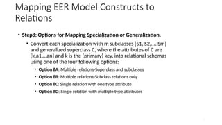
• Step8: Options for Mapping Specialization or Generalization.
• Convert each specialization with m subclasses {S1, S2,….,Sm}
and generalized superclass C, where the attributes of C are
{k,a1,…an} and k is the (primary) key, into relational schemas
using one of the four following options:
• Option 8A: Multiple relations-Superclass and subclasses
• Option 8B: Multiple relations-Subclass relations only
• Option 8C: Single relation with one type attribute
• Option 8D: Single relation with multiple type attributes

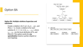
39. Option 8A
Option 8A: Multiple relations-Superclass and
subclasses
Create a relation L for C as L{k,a1,…an}, and
PK(L) = k. Create a relation Li for each
subclass Si, 1 < i < m, Li{k, si1,…,siik}, where
si1,…,siik are the local attributes of Si, and
PK(Li)=k. This option works for any
specialization (total or partial, disjoint or
over-lapping).

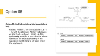
40. Option 8B
Option 8B: Multiple relations-Subclass relations
only
Create a relation Li for each subclass Si, 1 < i
< m, with the attributes Attr(Li) = {attributes
of Si} U {k,a1…,an} and PK(Li) = k. This
option only works for a specialization whose
subclasses are total (every entity in the
superclass must belong to (at least) one of
the subclasses).

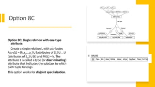
41. Option 8C
Option 8C: Single relation with one type
attribute.
Create a single relation L with attributes
Attrs(L) = {k,a1,…an} U {attributes of S1} U…U
{attributes of Sm} U {t} and PK(L) = k. The
attribute t is called a type (or discriminating)
attribute that indicates the subclass to which
each tuple belongs.
This option works for disjoint specilaization.

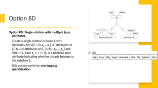
42. Option 8D
Option 8D: Single relation with multiple type
attributes.
Create a single relation schema L with
attributes Attrs(L) = {k,a1,…an} U {attributes of
S1} U…U {attributes of Sm} U {t1, t2,…,tm} and
PK(L) = k. Each ti, 1 < I < m, is a Boolean type
attribute indicating whether a tuple belongs to
the subclass Si.
This option works for overlapping
specilaization.

43. 43
Mapping EER Model Constructs to
Relations (cont)
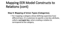
Step 9: Mapping of Union Types (Categories).
• For mapping a category whose defining superclass have
different keys, it is customary to specify a new key attribute,
called a surrogate key, when creating a relation to
correspond to the category.

44. 44
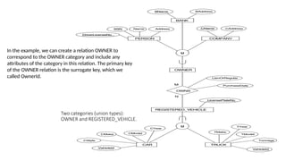
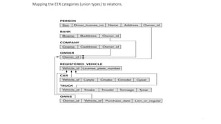
Two categories (union types):
OWNER and REGISTERED_VEHICLE.
In the example, we can create a relation OWNER to
correspond to the OWNER category and include any
attributes of the category in this relation. The primary key
of the OWNER relation is the surrogate key, which we
called OwnerId.

45. 45
Mapping the EER categories (union types) to relations.

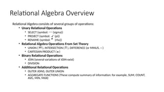
46. Relational Algebra Overview
Relational Algebra consists of several groups of operations:
• Unary Relational Operations
• SELECT (symbol:  (sigma))
• PROJECT (symbol:  (pi))
• RENAME (symbol:  (rho))
• Relational Algebra Operations From Set Theory
• UNION (  ), INTERSECTION (  ), DIFFERENCE (or MINUS, – )
• CARTESIAN PRODUCT ( x )
• Binary Relational Operations
• JOIN (several variations of JOIN exist)
• DIVISION
• Additional Relational Operations
• OUTER JOINS, OUTER UNION
• AGGREGATE FUNCTIONS (These compute summary of information: for example, SUM, COUNT,
AVG, MIN, MAX)

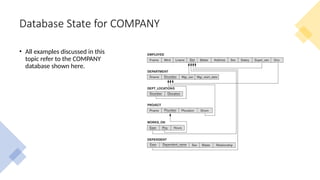
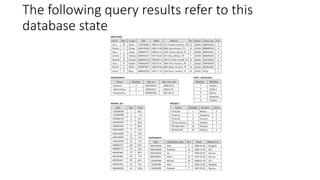
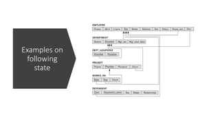
47. Database State for COMPANY
• All examples discussed in this
topic refer to the COMPANY
database shown here.

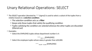
48. Unary Relational Operations: SELECT
• The SELECT operation (denoted by  (sigma)) is used to select a subset of the tuples from a
relation based on a selection condition.
• The selection condition acts as a filter
• Keeps only those tuples that satisfy the qualifying condition
• Tuples satisfying the condition are selected whereas the other tuples are discarded
(filtered out)
• Examples:
• Select the EMPLOYEE tuples whose department number is 4:
 DNO = 4 (EMPLOYEE)
• Select the employee tuples whose salary is greater than $30,000:
 SALARY > 30,000 (EMPLOYEE)

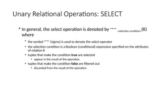
49. Unary Relational Operations: SELECT
• In general, the select operation is denoted by  <selection condition>(R)
where
• the symbol (sigma) is used to denote the select operator
• the selection condition is a Boolean (conditional) expression specified on the attributes
of relation R
• tuples that make the condition true are selected
• appear in the result of the operation
• tuples that make the condition false are filtered out
• discarded from the result of the operation

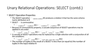
50. Unary Relational Operations: SELECT (contd.)
• SELECT Operation Properties
• The SELECT operation  <selection condition>(R) produces a relation S that has the same schema
(same attributes) as R
• SELECT  is commutative:
•  <condition1>( < condition2> (R)) =  <condition2> ( < condition1> (R))
• Because of commutativity property, a cascade (sequence) of SELECT operations may be
applied in any order:
• <cond1>(<cond2> (<cond3> (R)) = <cond2> (<cond3> (<cond1> ( R)))
• A cascade of SELECT operations may be replaced by a single selection with a conjunction of all
the conditions:
• <cond1>(< cond2> (<cond3>(R)) = <cond1> AND < cond2> AND < cond3>(R)))
• The number of tuples in the result of a SELECT is less than (or equal to) the number of
tuples in the input relation R

51. The following query results refer to this
database state

52. Unary Relational Operations: SELECT (contd.)
• Examples:
Select the EMPLOYEE tuples whose department number is 4 with salary greater than 25000 or
department number is 5 with salary greater than 30000 :
 (DNO = 4 AND Salary>25000) OR (DNO = 5 AND Salary>30000) (EMPLOYEE)

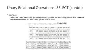
53. Unary Relational Operations: PROJECT
• PROJECT Operation is denoted by  (pi)
• This operation keeps certain columns (attributes) from a relation and
discards the other columns.
• PROJECT creates a vertical partitioning
• The list of specified columns (attributes) is kept in each tuple
• The other attributes in each tuple are discarded
• Example: To list each employee’s first and last name and salary, the
following is used:
LNAME, FNAME,SALARY(EMPLOYEE)

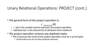
54. Unary Relational Operations: PROJECT (cont.)
• The general form of the project operation is:
<attribute list>(R)
•  (pi) is the symbol used to represent the project operation
• <attribute list> is the desired list of attributes from relation R.
• The project operation removes any duplicate tuples
• This is because the result of the project operation must be a set of tuples
• Mathematical sets do not allow duplicate elements.

55. Unary Relational Operations: PROJECT
(contd.)
• PROJECT Operation Properties
• The number of tuples in the result of projection <list>(R) is always less or
equal to the number of tuples in R
•  <list1> ( <list2> (R) ) =  <list1> (R) as long as <list2> contains the attributes in
<list1>
• PROJECT is not commutative

56. Unary Relational Operations: PROJECT
(contd.)
• Example: To list each employee’s first and last name and salary, the
following is used:
LNAME, FNAME,SALARY(EMPLOYEE)

57. Relational Algebra Expressions
• We may want to apply several relational algebra operations one after
the other
• Either we can write the operations as a single relational algebra expression
by nesting the operations, or
• We can apply one operation at a time and create intermediate result
relations.
• In the latter case, we must give names to the relations that hold
the intermediate results.

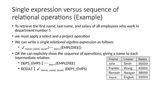
58. Single expression versus sequence of
relational operations (Example)
• To retrieve the first name, last name, and salary of all employees who work in
department number 5
• we must apply a select and a project operation
• We can write a single relational algebra expression as follows:
• FNAME, LNAME, SALARY( DNO=5(EMPLOYEE))
• OR We can explicitly show the sequence of operations, giving a name to each
intermediate relation:
• DEP5_EMPS   DNO=5(EMPLOYEE)
• RESULT   FNAME, LNAME, SALARY (DEP5_EMPS)

59. Unary Relational Operations: RENAME
• The RENAME operator is denoted by  (rho)
• In some cases, we may want to rename the attributes of a relation or
the relation name or both
• Useful when a query requires multiple operations
• Necessary in some cases (see JOIN operation later)

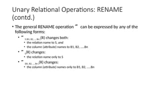
60. Unary Relational Operations: RENAME
(contd.)
• The general RENAME operation  can be expressed by any of the
following forms:
• S (B1, B2, …, Bn )(R) changes both:
• the relation name to S, and
• the column (attribute) names to B1, B2, …..Bn
• S(R) changes:
• the relation name only to S
• (B1, B2, …, Bn )(R) changes:
• the column (attribute) names only to B1, B2, …..Bn

61. Relational Algebra Operations from Set Theory:
UNION
• Binary operation, denoted by 
• The result of R  S, is a relation that includes all tuples that are either in R or
in S or in both R and S
• Duplicate tuples are eliminated
• The two-operand relations R and S must be “type compatible” (or UNION
compatible)
• R and S must have same number of attributes
• Each pair of corresponding attributes must be type compatible (have same or
compatible domains)

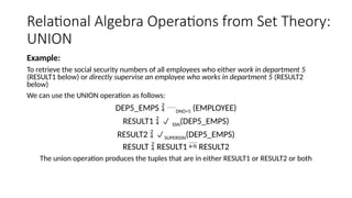
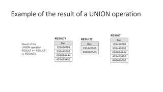
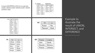
62. Relational Algebra Operations from Set Theory:
UNION
Example:
To retrieve the social security numbers of all employees who either work in department 5
(RESULT1 below) or directly supervise an employee who works in department 5 (RESULT2
below)
We can use the UNION operation as follows:
DEP5_EMPS  DNO=5 (EMPLOYEE)
RESULT1   SSN(DEP5_EMPS)
RESULT2  SUPERSSN(DEP5_EMPS)
RESULT  RESULT1  RESULT2
The union operation produces the tuples that are in either RESULT1 or RESULT2 or both

63. Example of the result of a UNION operation

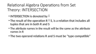
64. Relational Algebra Operations from Set
Theory: INTERSECTION
• INTERSECTION is denoted by 
• The result of the operation R  S, is a relation that includes all
tuples that are in both R and S
• The attribute names in the result will be the same as the attribute
names in R
• The two operand relations R and S must be “type compatible”

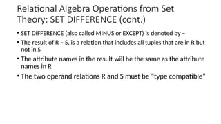
65. Relational Algebra Operations from Set
Theory: SET DIFFERENCE (cont.)
• SET DIFFERENCE (also called MINUS or EXCEPT) is denoted by –
• The result of R – S, is a relation that includes all tuples that are in R but
not in S
• The attribute names in the result will be the same as the attribute
names in R
• The two operand relations R and S must be “type compatible”

66. Example to
illustrate the
result of UNION,
INTERSECT, and
DIFFERENCE

67. Some properties of UNION, INTERSECT, and
DIFFERENCE
• Notice that both union and intersection are commutative operations; that is
• R  S = S  R, and R  S = S  R
• Both union and intersection can be treated as n-ary operations applicable to any
number of relations as both are associative operations; that is
• R  (S  T) = (R  S)  T
• (R  S)  T = R  (S  T)
• The minus operation is not commutative; that is, in general
• R – S ≠ S – R

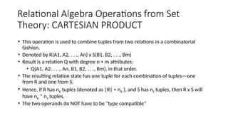
68. Relational Algebra Operations from Set
Theory: CARTESIAN PRODUCT
• This operation is used to combine tuples from two relations in a combinatorial
fashion.
• Denoted by R(A1, A2, . . ., An) x S(B1, B2, . . ., Bm)
• Result is a relation Q with degree n + m attributes:
• Q(A1, A2, . . ., An, B1, B2, . . ., Bm), in that order.
• The resulting relation state has one tuple for each combination of tuples—one
from R and one from S.
• Hence, if R has nR tuples (denoted as |R| = nR ), and S has nS tuples, then R x S will
have nR * nS tuples.
• The two operands do NOT have to be "type compatible”

69. Relational Algebra Operations from Set
Theory: CARTESIAN PRODUCT (cont.)
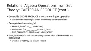
• Generally, CROSS PRODUCT is not a meaningful operation
• Can become meaningful when followed by other operations
• Example (not meaningful):
• FEMALE_EMPS   SEX=’F’(EMPLOYEE)
• EMPNAMES   FNAME, LNAME, SSN (FEMALE_EMPS)
• EMP_DEPENDENTS  EMPNAMES x DEPENDENT
• EMP_DEPENDENTS will contain every combination of EMPNAMES and
DEPENDENT
• whether or not they are actually related

70. Relational Algebra Operations from Set
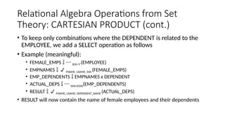
Theory: CARTESIAN PRODUCT (cont.)
• To keep only combinations where the DEPENDENT is related to the
EMPLOYEE, we add a SELECT operation as follows
• Example (meaningful):
• FEMALE_EMPS   SEX=’F’(EMPLOYEE)
• EMPNAMES   FNAME, LNAME, SSN (FEMALE_EMPS)
• EMP_DEPENDENTS  EMPNAMES x DEPENDENT
• ACTUAL_DEPS   SSN=ESSN(EMP_DEPENDENTS)
• RESULT   FNAME, LNAME, DEPENDENT_NAME (ACTUAL_DEPS)
• RESULT will now contain the name of female employees and their dependents

71. Example of applying CARTESIAN PRODUCT

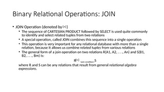
72. Binary Relational Operations: JOIN
• JOIN Operation (denoted by )
• The sequence of CARTESIAN PRODUCT followed by SELECT is used quite commonly
to identify and select related tuples from two relations
• A special operation, called JOIN combines this sequence into a single operation
• This operation is very important for any relational database with more than a single
relation, because it allows us combine related tuples from various relations
• The general form of a join operation on two relations R(A1, A2, . . ., An) and S(B1,
B2, . . ., Bm) is:
R <join condition>S
where R and S can be any relations that result from general relational algebra
expressions.

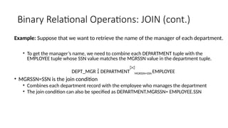
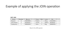
73. Binary Relational Operations: JOIN (cont.)
Example: Suppose that we want to retrieve the name of the manager of each department.
• To get the manager’s name, we need to combine each DEPARTMENT tuple with the
EMPLOYEE tuple whose SSN value matches the MGRSSN value in the department tuple.
DEPT_MGR  DEPARTMENT MGRSSN=SSN EMPLOYEE
• MGRSSN=SSN is the join condition
• Combines each department record with the employee who manages the department
• The join condition can also be specified as DEPARTMENT.MGRSSN= EMPLOYEE.SSN

74. Example of applying the JOIN operation

75. Some properties of JOIN
• Consider the following JOIN operation:
• R(A1, A2, . . ., An) S(B1, B2, . . ., Bm)
• Result is a relation Q with degree n + m attributes:
• Q(A1, A2, . . ., An, B1, B2, . . ., Bm), in that order.
• The resulting relation state has one tuple for each combination of tuples—r from R
and s from S, but only if they satisfy the join condition r[Ai]=s[Bj]
• Hence, if R has nR tuples, and S has nS tuples, then the join result will generally have
less than nR * nS tuples.
• Only related tuples (based on the join condition) will appear in the result
R.Ai=S.Bj

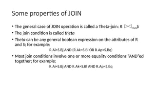
76. Some properties of JOIN
• The general case of JOIN operation is called a Theta-join: R S
• The join condition is called theta
• Theta can be any general boolean expression on the attributes of R
and S; for example:
R.Ai<S.Bj AND (R.Ak=S.Bl OR R.Ap<S.Bq)
• Most join conditions involve one or more equality conditions “AND”ed
together; for example:
R.Ai=S.Bj AND R.Ak=S.Bl AND R.Ap=S.Bq
theta

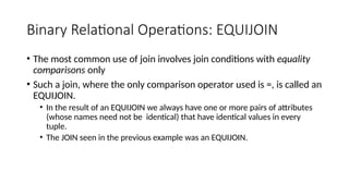
77. Binary Relational Operations: EQUIJOIN
• The most common use of join involves join conditions with equality
comparisons only
• Such a join, where the only comparison operator used is =, is called an
EQUIJOIN.
• In the result of an EQUIJOIN we always have one or more pairs of attributes
(whose names need not be identical) that have identical values in every
tuple.
• The JOIN seen in the previous example was an EQUIJOIN.

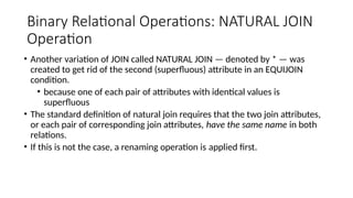
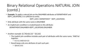
78. Binary Relational Operations: NATURAL JOIN
Operation
• Another variation of JOIN called NATURAL JOIN — denoted by * — was
created to get rid of the second (superfluous) attribute in an EQUIJOIN
condition.
• because one of each pair of attributes with identical values is
superfluous
• The standard definition of natural join requires that the two join attributes,
or each pair of corresponding join attributes, have the same name in both
relations.
• If this is not the case, a renaming operation is applied first.

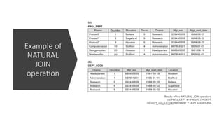
79. Binary Relational Operations NATURAL JOIN
(contd.)
• Example: To apply a natural join on the DNUMBER attributes of DEPARTMENT and
DEPT_LOCATIONS, it is sufficient to write:
DEPT_LOCS  DEPARTMENT * DEPT_LOCATIONS
• Only attribute with the same name is DNUMBER
• An implicit join condition is created based on this attribute:
DEPARTMENT.DNUMBER=DEPT_LOCATIONS.DNUMBER
• Another example: Q  R(A,B,C,D) * S(C,D,E)
• The implicit join condition includes each pair of attributes with the same name, “AND”ed
together:
• R.C=S.C AND R.D=S.D
• Result keeps only one attribute of each such pair:
• Q(A,B,C,D,E)

80. Example of
NATURAL
JOIN
operation

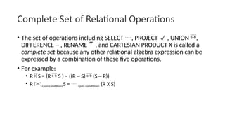
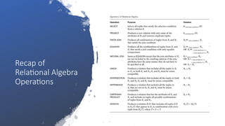
81. Complete Set of Relational Operations
• The set of operations including SELECT , PROJECT  , UNION ,
DIFFERENCE - , RENAME , and CARTESIAN PRODUCT X is called a
complete set because any other relational algebra expression can be
expressed by a combination of these five operations.
• For example:
• R  S = (R  S ) – ((R - S)  (S - R))
• R <join condition>S =  <join condition> (R X S)

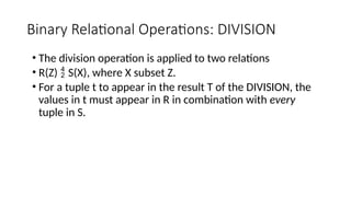
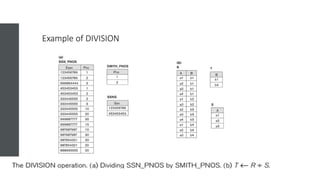
82. Binary Relational Operations: DIVISION
• The division operation is applied to two relations
• R(Z)  S(X), where X subset Z.
• For a tuple t to appear in the result T of the DIVISION, the
values in t must appear in R in combination with every
tuple in S.

83. Example of DIVISION

84. Recap of
Relational Algebra
Operations

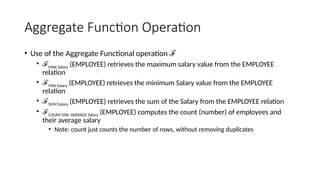
85. Additional Relational Operations: Aggregate
Functions and Grouping
• A type of request that cannot be expressed in the basic relational algebra is to
specify mathematical aggregate functions on collections of values from the
database.
• Examples of such functions include retrieving the average or total salary of all
employees or the total number of employee tuples.
• These functions are used in simple statistical queries that summarize information
from the database tuples.
• Common functions applied to collections of numeric values include
• SUM, AVERAGE, MAXIMUM, and MINIMUM.
• The COUNT function is used for counting tuples or values.

86. Aggregate Function Operation
• Use of the Aggregate Functional operation ℱ
• ℱMAX Salary (EMPLOYEE) retrieves the maximum salary value from the EMPLOYEE
relation
• ℱMIN Salary (EMPLOYEE) retrieves the minimum Salary value from the EMPLOYEE
relation
• ℱSUM Salary (EMPLOYEE) retrieves the sum of the Salary from the EMPLOYEE relation
• ℱCOUNT SSN, AVERAGE Salary (EMPLOYEE) computes the count (number) of employees and
their average salary
• Note: count just counts the number of rows, without removing duplicates

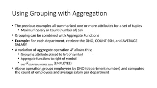
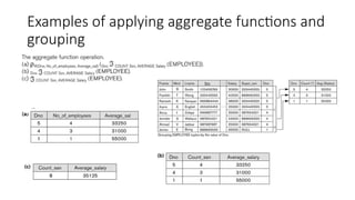
87. Using Grouping with Aggregation
• The previous examples all summarized one or more attributes for a set of tuples
• Maximum Salary or Count (number of) Ssn
• Grouping can be combined with Aggregate Functions
• Example: For each department, retrieve the DNO, COUNT SSN, and AVERAGE
SALARY
• A variation of aggregate operation allows this:
ℱ
• Grouping attribute placed to left of symbol
• Aggregate functions to right of symbol
• DNO ℱCOUNT SSN, AVERAGE Salary (EMPLOYEE)
• Above operation groups employees by DNO (department number) and computes
the count of employees and average salary per department

88. Examples of applying aggregate functions and
grouping

89. Additional Relational Operations
• The OUTER JOIN Operation
• In NATURAL JOIN and EQUIJOIN, tuples without a matching (or related) tuple are
eliminated from the join result
• Tuples with null in the join attributes are also eliminated
• This amounts to loss of information.
• A set of operations, called OUTER joins, can be used when we want to keep all the
tuples in R, or all those in S, or all those in both relations in the result of the join,
regardless of whether or not they have matching tuples in the other relation.

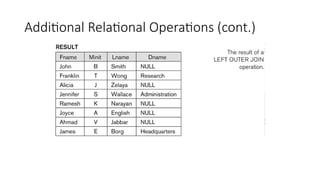
90. Additional Relational Operations (cont.)
• The left outer join operation keeps every tuple in the first or left
relation R in R S; if no matching tuple is found in S, then the
attributes of S in the join result are filled or “padded” with null values.
• A similar operation, right outer join, keeps every tuple in the second
or right relation S in the result of R S.
• A third operation, full outer join, denoted by keeps all tuples
in both the left and the right relations when no matching tuples are
found, padding them with null values as needed.

91. Additional Relational Operations (cont.)

92. Examples on
following
state

93. Query 1. Retrieve the name and address of all employees who work for
the ‘Research’ department.
Can also be written in single line:

94. Query 2. For every project located in ‘Stafford’, list the project number,
the controlling department number, and the department manager’s
last name, address, and birth date.