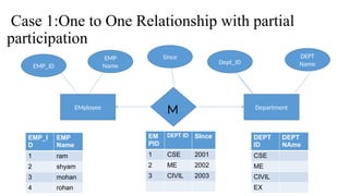
Database Management
System (DBMS)
Dr. Amit K. (AI Researcher)
Assistant Professor - VIT Bhopal Uni
Relational Model
•Relational Model was proposed by E.F. Codd to model data in the form of
relations or tables, where all data is represented in terms of tuples, grouped
into relations.
•A database organized in terms of the relational model is a relational
database.
•The purpose of the relational model is to provide a declarative method for
specifying data and queries: users directly state what information the
database contains and what information they want from it, and let the
database management system software take care of describing data
structures for storing the data and retrieval procedures for answering
queries.
Relational Table
Student
• ROLL_NO NAME ADDRESS PHONE AGE
1 RAM DELHI 94551234511 18
2 RAMESH GURGAON 96524315431
83 3 SUJIT ROHTAK
91562531311 20 4 SURESH
DELHI 67845399120 18
• Attribute: Attributes are the properties that define a relation. e.g.; ROLL_NO, NAME
• Relation Schema: A relation schema represents name of the relation with its attributes.
e.g.; STUDENT (ROLL_NO, NAME, ADDRESS, PHONE and AGE) is relation schema
for STUDENT. If a schema has more than 1 relation, it is called Relational Schema.
• Tuple: Each row in the relation is known as tuple. The above relation contains 4 tuples
• Relation Instance: The set of tuples of a relation at a particular instance of time is called
as relation instance. Table 1 shows the relation instance of STUDENT at a particular
time. It can change whenever there is insertion, deletion or updation in the database.
• Degree: The number of attributes in the relation is known as degree of the relation.
The STUDENT relation defined above has degree 5.
• Cardinality: The number of tuples in a relation is known as cardinality.
The STUDENT relation defined above has cardinality 4.
• Column: Column represents the set of values for a particular attribute. The
column ROLL_NO is extracted from relation STUDENT.
ER Vs Relational Model
ER Model Relational Model
ER model is the high level or conceptual model It is the representational or implementation model.
It represents collection of entities and describes
relationship between them.
It represent data in the form of tables and describes
relationship between them
It is used by people who don’t know how database is
implemented
It is used by programmers.
It consists of components like Entity, Entity Type,
Entity Set
It consists of components like domain, attributes,
tuples.
It is easy to understand the relationship between
entities
It is less easy to derive the relationship between
different tables.
Key
• Set of attribute by which each tuple of a relational table can be
uniquely identified.
• Types of Keys:
❑Super Key
❑Candidate Key
❑Primary Key
❑Alternate Key
Keys
• SUPER KEYS:
Any set of attributes that allows us to identify unique rows (tuples) in a
given relation are known as super keys. Or Superset of any candidate key
is a super key.
• Candidate Key: A super key whose proper subset is not a super key is the
candidate key. Also we can say, Minimal Super key is the candidate Key.
• Primary Key: A Candidate Key whose value can not be null is the primary
key.
• Alternate Key: Keys which are candidate key and not primary key are the
alternate keys.
Super Key and Candidate Key
X A B C
1 2 2 5
2 2 3 3
3 1 4 4
4 1 1 5
5 3 6 7
6 3 6 6
7 4 Null 8
Super Keys: { X, BC,AC,XA,XB,XC,ABC,XAB,XBC,XAC}
Candidate: {X,BC,AC}
Primary Key: {X,AC}
Alternate Key : BC
EMP_ID EMP
NAme
Address
1 Ram
2 shyam
3 Aman
EMP ID DEPT ID SInce
2 CSE 2002
2 ME 2006
1 Civil 2001
3 CSE 2000
Referenced Relation (Employee) Referencing Relation (works on) Referenced Relation (Department)
Works
On
Employee Department
DEPT
ID
Number of
Employee
CSE 202
ME 246
Civil 262
EMP _ID and DEPT ID in the “works on” relation are the foreign keys.
Foreign Key
Set of attribute that references to primary key of the Same or some other relation
Constraints in Relational Model
• While designing Relational Model, we define some conditions which
must hold for data present in database are called Constraints. These
constraints are checked before performing any operation (insertion,
deletion and updation) in database. If there is a violation in any of
constrains, operation will fail.
• Domain Constraints: These are attribute level constraints. An
attribute can only take values which lie inside the domain range. e.g,;
If a constrains AGE>0 is applied on STUDENT relation, inserting
negative value of AGE will result in failure.
• Key Integrity: Every relation in the database should have atleast one
set of attributes which defines a tuple uniquely. Those set of
attributes is called key. e.g.; ROLL_NO in STUDENT is a key. No two
students can have same roll number. So a key has two properties:
• It should be unique for all tuples.
• It can’t have NULL values.
Referential Integrity:
• When one attribute of a relation can only take values from other
attribute of same relation or any other relation, it is called referential
integrity. Let us suppose we have 2 relations.
• EMP ID of Works ON can only take the values which are present in
EMP ID of Employee which is called referential integrity constraint.
The relation which is referencing to other relation is called
REFERENCING RELATION (“Works On” in this case) and the relation to
which other relations refer is called REFERENCED RELATION
(Employee in this case).
EMP_ID EMP
NAme
Address
1 Ram
2 shyam
3 Aman
EMP ID DEPT ID SInce
2 CSE 2002
2 ME 2006
1 Civil 2001
8 CSE 2000
Referenced Relation Employee) Referencing Relation “works on” Referenced Relation “ Department”
Works
On
Employee Department
DEPT
ID
Number of
Employee
CSE 202
ME 246
Civil 262
EMP _ID and DEPT ID in the “works on” relation are the foreign keys.
Foreign Key
Set of attribute that references to primary key of the Same or some other relation
ANOMALIES
• An anomaly is an irregularity, or something which deviates from the
expected or normal state. When designing databases, we identify
three types of anomalies: Insert, Update and Delete.
• Insertion Anomaly in Referencing Relation:
We can’t insert a row in REFERENCING RELATION if referencing
attribute’s value is not present in referenced attribute value.
• Deletion/ Updation Anomaly in Referenced Relation:
We can’t delete or update a row from REFERENCED RELATION if
value of REFRENCED ATTRIBUTE is used in value of
REFERENCING ATTRIBUTE.
• ON DELETE CASCADE: It will delete the tuples from REFERENCING
RELATION if value used by REFERENCING ATTRIBUTE is deleted
from REFERENCED RELATION. e.g;, if we delete a row from BRANCH
with BRANCH_CODE ‘CS’, the rows in STUDENT relation with
BRANCH_CODE CS (ROLL_NO 1 and 2 in this case) will be deleted.
• ON UPDATE CASCADE: It will update the REFERENCING
ATTRIBUTE in REFERENCING RELATION if attribute value used by
REFERENCING ATTRIBUTE is updated in REFERENCED RELATION.
e.g;, if we update a row from BRANCH with BRANCH_CODE ‘CS’ to
‘CSE’, the rows in STUDENT relation with BRANCH_CODE CS
(ROLL_NO 1 and 2 in this case) will be updated with BRANCH_CODE
‘CSE’.
Minimization of ER Diagram and
Conversion of ER diagram to Relational
Tables
ER Diagram Minimization
Case 1:One to One Relationship with partial
participation
EMployee Department
M
EMP_ID
EMP
Name
Dept_ID
DEPT
Name
EMP_I
D
EMP
Name
1 ram
2 shyam
3 mohan
4 rohan
EM
PID
DEPT ID SInce
1 CSE 2001
2 ME 2002
3 CIVIL 2003
DEPT
ID
DEPT
NAme
CSE
ME
CIVIL
EX
Since
Minimum Number of Tables Required
EMP_ID EMP Name Dept ID DEPt Name SInce
1 ram CSE Computer Scince
Engineering
2001
2 shyam ME Machanical
ENgineering
2002
3 mohan CIVIL Civil ENgineering 2003
4 rohan NUll NUll NULL
Null NUll EC Electronics and
Communication
Null
We can not merge all tables into a single table as all attribute will have null values thus we can not make ant attribute a
primary key
Minimum 2 Tables required when both entities
are partially participated in 1:1 relationship
EMP_ID EMP Name
1 ram
2 shyam
3 mohan
4 rohan
Dept
ID
DEPt Name SInce EMP ID
CSE Computer
Scince
Engineering
2001 1
ME Machanical
ENgineering
2002 2
CIVIL Civil
ENgineering
2003 3
EC Electronics
and
Communicatio
n
Null Null
Department + M
EMPLOYEE
We can merge either of the participated entity with the relation. Here the department is merged with
the relation.
Minimum 2 tables are required
EMP_ID EMP
Name
SInce Dept ID
1 ram 2001 CSE
2 shyam 2002 ME
3 mohan 2003 CIVIL
4 rohan NULL
Dept ID DEPt Name
CSE Computer Scince Engineering
ME Machanical ENgineering
CIVIL Civil ENgineering
EC Electronics and
Communication
Employee + M
Department
Case 2:One to One relationship with at least
one total participation
EMployee Department
M
EMP_ID
EMP
Name
Dept_ID
DEPT
Name
EMP_I
D
EMP
Name
1 ram
2 shyam
3 mohan
4 rohan
EM
PID
DEPT ID SInce
1 CSE 2001
2 ME 2002
3 CIVIL 2003
DEPT
ID
DEPT
NAme
CSE
ME
CIVIL
Since
Minimum 1Table required when at least one
total participation
EMP_ID EMP Name Dept ID DEPt Name SInce
1 ram CSE Computer Scince
Engineering
2001
2 shyam ME Machanical
ENgineering
2002
3 mohan CIVIL Civil ENgineering 2003
4 rohan NUll NUll NULL
Many to One Relationship
Employee
Department
M
EMP_ID
EMP
Name
Dept_ID
DEPT
Name
EMP_I
D
EMP
Name
1 ram
2 shyam
3 mohan
4 rohan
5 sohan
EM
PID
DEPT ID SInce
1 CSE 2001
2 ME 2002
3 CIVIL 2003
4 ME 2000
DEPT ID DEPT
NAme
Number of
Emplyee
CSE
ME
CIVIL
Architectur
e
Since
Minimum 2 tables are required in M:1 relationship
EMP_ID EMP
Name
SInce Dept ID
1 ram 2001 CSE
2 shyam 2002 ME
3 mohan 2003 CIVIL
4 rohan 2000 ME
Dept ID DEPt Name
CSE Computer Science Engineering
ME Mechanical Engineering
CIVIL Civil Engineering
EC Electronics and
Communication
If we merge the side of “many “ with the relationship then repetition will not occur, therefore we can merge the
side of ‘many” with the relationship in case of many to one.
Repetition will occur if we merge side of “one” with a relationship,
therefore we can’t merge the side of “many” with the relationship.
EMP_ID EMP Name
1 ram
2 shyam
3 mohan
4 rohan
Number of
Employee
Dept
ID
DEPt Name SInce EMP ID
20 CSE Computer Scince
Engineering
2001 1
18 ME Machanical ENgineering 2002 2
122 CIVIL Civil ENgineering 2003 3
18 ME Mechanical Engineering 2000 4
Many to Many Relationship
We can not merge tables in case of Many to many relationship
IF we try to merge tables in Many to many
relationship then redundancy will occur
Std ID STD Name Course ID Course name
1 A c1 z
1 A c2 y
2 B c1 z
2 B c2 y
Student+ENrollment
Question
For Student(SID, Name), SID is the primary key. For Course(CID, C_name ), CID is the primary key
Now the question is, what should be the primary key for Enroll? Should it be SID or CID or both
combined into one.
Question
Now the question is, what should be the primary key for Enroll? Should it be SID or CID or both
combined into one.
Question
• A1 and B1 are primary keys of E1 and E2 respectively. Now the
question is, what should be the primary key for R?
Mapping of ER diagram to Relational Tables
Employee
EMP_ID
Dependent
Dependent Name
Dependent Address
Phone Number
N
Department
M
N
Works
On
Dependency
Project
Project Start Date
N
Project ID
Department ID
Since
Project
Allotment
Age
Address
city
Street
The basic rule for converting the ER diagrams into tables is
•Convert all the Entities in the diagram to tables.
All the entities represented in the rectangular box in the ER diagram become independent
tables in the database. In the below diagram, Employee, Department, Dependent, project
forms individual tables.
•All single valued attributes of an entity is converted to a column of the table
•Key attribute in the ER diagram becomes the Primary key of the table.
•Declare the foreign key column, if applicable.
•Any multi-valued attributes are converted into new table.
•A phone number in the Employee table is a multivalued attribute. Any employee can
have any number of phone number. So we cannot represent multiple values in a single
column of Employee table. We need to store it separately, so that we can store any
number of phone numbers, adding/ removing / deleting phone numbers should not create
any redundancy or anomalies in the system.
• we create a separate table STUD_PHN with EMP_ID and Phn_No as its columns.
We create a composite key using both the columns.
• Any composite attributes are merged into same table as different columns.
• In the diagram above, Employee Address is a composite attribute. It has Door#,
Street, City. These attributes are merged into EMPLOYEE table as individual
columns.
• Converting Weak Entity: Weak entity is also represented as table. All the
attributes of the weak entity forms the column of the table. But the key attribute
represented in the diagram cannot form the primary key of this table. We have to
add a foreign key column, which would be the primary key column of its strong
entity. This foreign key column along with its key attribute column forms the
primary key of the table.
• Create table correspond to each relationship.
• Add primary key attributes of the participated entities as columns in the relationship.
• If relationship is one to one and both have partial participation then merge one of
the entity with the relationship, i.e. merge table of one of the participant entity and
the relationship into a single table
• If relationship is one to one and at least one have total participation then merge the
relations of both entities and relationship.
• If Relationship is many to one then merge relationship with the participated entity
that belongs to “many” side.
• If relationship is many to many then don’t do minimization.
Emp ID Name Age DOB Phone
Numbe
r
1 SOhan 34 1986 463245
1 SOhan 34 1986 769313
1 SOhan 34 1986 421456
Emp ID Name Age DOB
1 SOhan 34 1986
2 Mohan 40 1982
3 ROhan 36 1983
Emp ID Phone
Numbe
r
1 463245
1 769313
1 421456
2 674217
2 43245
Example of Multivalued Attribute:
Referencing Relation
Referenced Relation
Dependent
Name
Age Workin
g
Status
SOhan 34 Workin
g
SOhan 30 Not
working
Mohan 36 Not
working
Emp ID Dependent
Name
1 SOhan
2 SOhan
1 Mohan
Emp
ID
Name Age DOB Phone
Number
1 John 34 198
6
463245
2 Tom 34 198
6
769313
3 Alice 34 198
6
421456
Employee
Dependency Dependent (weak Entity)
Emp
ID
Name Age DOB Phone
Number
1 John 34 198
6
463245
2 Tom 34 198
6
769313
3 Alice 34 198
6
421456
Emp ID Dependent
Name
Age Working
Status
1 Sohan 30 Not working
2 Sohan 34 working
1 Mohan 36 Not working
Example of Weak Entity:
New Table
Employee
EMPID
Emp Name
Age
Street
City
Works On
Emp ID (foreign Key)
Dept ID (foreign key)
Since
Dependency
Emp ID ( foreign Key)
Dependent Name
Department
Dept _ID
Number of Employee
Project
Project ID
Project Start Date
Project Allotment
Emp ID ( foreign Key)
Project ID( foreign Key)
Dependent
Dependent Name
Age
Working status
Employee-Phn No
Emp ID ( foreign Key)
Phn No
Employee-project
Allotment
EMPID
Emp Name
Age
Street
City
Project ID (foreign Key)
Works On
Emp ID (foreign Key)
Dept ID (foreign key)
Since
Employee-Phn No
Emp ID (foreign Key)
Phone Number
Employee Dependent
Dependent Name
Emp ID ( foreign Key)
Age
Working Status
Department
Dept _ID
Number of Employee
Project
Project ID
Project Start Date
Relation Algebra
• Procedural Query Languages.
• The basic set of operations for the formal relational model is the relational
algebra.
• These operations enable a user to specify basic retrieval requests as relational
algebra expressions.
• The result of a retrieval query is a new relation.
Relation Algebra
• The algebra operations thus produce new relations, which can be further
manipulated using operations of the same algebra.
• A sequence of relational algebra operations forms a relational algebra
expression, whose result will also be a relation that represents the result of a
database query (or retrieval request).
Fundamental Operators
• Unary relation operation
• Operate on single relation.
• Two types:
• Selection (σ)
• Projection (π)
Selection (σ)
• choose a subset of the tuples from a relation that satisfies a selection condition.
• For example, to select the EMPLOYEE tuples whose department is 4, or those whose salary is
greater than $30,000, we can individually specify each of these two conditions with a SELECT
operation as follows:
σDno=4(EMPLOYEE)
σSalary>30000(EMPLOYEE)
• In general, the SELECT operation is denoted by
σ<selection condition>(R)
• where the symbol σ (sigma) is used to denote the SELECT operator and the selection condition
is a Boolean expression (condition) specified on the attributes of relation R. Notice that R is
generally a relational algebra expression whose result is a relation—the simplest such expression
is just the name of a database relation. The relation resulting from the SELECT operation has the
same attributes as R.
Selection (σ)
• The Boolean expression specified in <selection condition> is made up of a number of
clauses of the form
<attribute name> <comparison op> <constant value>
or
<attribute name> <comparison op> <attribute name
• where <attribute name> is the name of an attribute of R, <comparison op> is normally one
of the operators {=, <, ≤, >, ≥, ≠}, and <constant value> is a constant value from the
attribute domain. Clauses can be connected by the standard Boolean operators and, or, and
not to form a general selection condition. For example, to select the tuples for all employees
who either work in department 4 and make over $25,000 per year, or work in department 5
and make over $30,000, we can specify the following SELECT operation:
σ(Dno=4 AND Salary>25000) OR (Dno=5 AND Salary>30000)(EMPLOYEE)
Projection (π)
• Selects certain columns from the table and discards the other columns.
• For example, to list each employee’s first and last name and salary, we can use
the PROJECT operation as follows:
πLname, Fname, Salary(EMPLOYEE)
• The general form of the PROJECT operation is π<attribute list>(R)
• where π (pi) is the symbol used to represent the PROJECT operation, and
<attribute list> is the desired sublist of attributes from the attributes of relation R.
• The result of the PROJECT operation has only the attributes specified in
<attribute list> in the same order as they appear in the list. Hence, its degree is
equal to the number of attributes in <attribute list>.
Projection (π)
• If the attribute list includes only nonkey attributes of R, duplicate tuples are
likely to occur.
• The PROJECT operation removes any duplicate tuples, so the result of the
PROJECT operation is a set of distinct tuples, and hence a valid relation. This is
known as duplicate elimination.
• For example, consider the following PROJECT operation:
• πSex, Salary(EMPLOYEE)
Sequences of Operations and the
RENAME Operation
For example, to retrieve the first name, last name, and salary of all employees who
work in department number 5, we must apply a SELECT and a PROJECT
operation. We can write a single relational algebra expression, also known as an in-
line expression, as follows:
πFname, Lname, Salary(σDno=5(EMPLOYEE))
Sequences of Operations
• Alternatively, we can explicitly show the sequence of operations, giving a name
to each intermediate relation, and using the assignment operation, denoted by ←
(left arrow), as follows:
1. DEP5_EMPS ← σDno=5(EMPLOYEE)
2. RESULT ← πFname, Lname, Salary(DEP5_EMPS)
RENAME Operation
1. TEMP ← σDno=5(EMPLOYEE)
2. R(First_name, Last_name, Salary) ← πFname, Lname, Salary(TEMP)
RENAME Operation
The general RENAME operation when applied to a relation R of degree n is
denoted by any of the following three forms:
ρS(B1, B2, ... , Bn)(R) or ρS(R) or ρ(B1, B2, ... , Bn)(R)
where,
The symbol ρ (rho) is used to denote the RENAME operator, S is the new relation
name, and B1, B2, … , Bn are the new attribute names.
The first expression renames both the relation and its attributes, the second renames
the relation only, and the third renames the attributes only.
Relational Algebra Operations from Set
Theory
• UNION, INTERSECTION, and MINUS Operations.
• For example, to retrieve the Social Security numbers of all employees who
either work in department 5 or directly supervise an employee who works in
department 5, we can use the UNION operation as follows:
1. DEP5_EMPS ← σDno=5(EMPLOYEE)
2. RESULT1 ← πSsn(DEP5_EMPS)
3. RESULT2(Ssn) ← πSuper_ssn(DEP5_EMPS)
4. RESULT ← RESULT1 RESULT2
∪
UNION, INTERSECTION, and MINUS
Operations
• Binary operations: each is applied to two sets (of tuples)
• Union compatibility or Type compatibility: When these operations are adapted
to relational databases, the two relations on which any of these three operations
are applied must have the same type of tuples.
• Two relations R(A1, A2, … , An) and S(B1, B2, … , Bn) are said to be union
compatible (or type compatible) if they have the same degree n and if dom(Ai)
= dom(Bi) for 1 ≤ i ≤ n.
• This means that the two relations have the same number of attributes and each
corresponding pair of attributes has the same domain.
UNION, INTERSECTION, and MINUS
Operations
• UNION: The result of this operation, denoted by R S, is a relation that
∪
includes all tuples that are either in R or in S or in both R and S. Duplicate
tuples are eliminated.
• INTERSECTION: The result of this operation, denoted by R ∩ S, is a relation
that includes all tuples that are in both R and S.
• SET DIFFERENCE (or MINUS): The result of this operation, denoted by R
– S, is a relation that includes all tuples that are in R but not in S.
The CARTESIAN PRODUCT (CROSS PRODUCT)
Operation
• CROSS JOIN (×)
• This set operation produces a new element by combining every member (tuple) from
one relation (set) with every member (tuple) from the other relation (set).
• The result of R(A1, A2, … , An) × S(B1, B2, … , Bm) is a relation Q with degree n + m
attributes Q(A1, A2, … , An, B1, B2, … , Bm), in that order.
• The resulting relation Q has one tuple for each combination of tuples—one from R
• and one from S. Hence, if R has nR tuples (denoted as |R| = nR), and S has nS tuples,
then R × S will have nR * nS tuples.
The CARTESIAN PRODUCT (CROSS PRODUCT)
Operation
1. FEMALE_EMPS ← σSex=‘F’(EMPLOYEE)
2. EMPNAMES ← πFname, Lname, Ssn(FEMALE_EMPS)
3. EMP_DEPENDENTS ← EMPNAMES × DEPENDENT
4. ACTUAL_DEPENDENTS ← σSsn=Essn(EMP_DEPENDENTS)
5. RESULT ← πFname, Lname,Dependent_name(ACTUAL_DEPENDENTS)
Binary Relational Operations: JOIN and
DIVISION
The JOIN Operation (⨝):
• Combine related tuples from two relations into single “longer” tuples.
• To illustrate JOIN, suppose that we want to retrieve the name of the manager of
each department. To get the manager’s name, we need to combine each
department tuple with the employee tuple whose Ssn value matches the Mgr_ssn
value in the department tuple. We do this by using the JOIN operation and then
projecting the result over the necessary attributes, as follows:
DEPT_MGR ← DEPARTMENT⨝Mgr_ssn=Ssn EMPLOYEE
RESULT ← πDname, Lname, Fname(DEPT_MGR)
• The JOIN operation can be specified as a CARTESIAN PRODUCT operation
followed by a SELECT operation.
DEPT_EMP← DEPARTMENT × EMPLOYEE
DEPT_MGR ← σMgr_ssn=Ssn(DEPT_EMP)
DName Dnumber Mgr_ssn . . . Fname Minit Lname Ssn . . .
Research 5 333445555 . . . Franklin T Wong 333445555 . . .
Administrati
on
4 987654321 . . . Jennifer S Wallace 987654321 . . .
Headquarte
rs
1 888665555 . . . James E Borg 888665555 . . .
• The general form of a JOIN operation on two relations R(A1, A2, … , An) and
S(B1, B2, … , Bm) is
R⨝<join condition>S
• A general join condition is of the form
<condition> AND <condition> AND … AND <condition>
• where each <condition> is of the form Ai θ Bj, Ai is an attribute of R, Bj is an
attribute of S, Ai and Bj have the same domain, and θ (theta) is one of the
comparison operators {=, <, ≤, >, ≥, ≠}. A JOIN operation with such a general
join condition is called a THETA JOIN.
• Tuples whose join attributes are NULL or for which the join condition is FALSE
do not appear in the result. In that sense, the JOIN operation does not
necessarily preserve all of the information in the participating relations, because
tuples that do not get combined with matching ones in the other relation do not
appear in the result.
Variations of JOIN
• EQUIJOIN: JOIN where the only comparison operator used is “=”.
• Result of an EQUIJOIN always have one or more pairs of attributes that
have identical values in every tuple.
• NATURAL JOIN(*): The standard definition of NATURAL JOIN requires that
the two join attributes (or each pair of join attributes) have the same name in
both relations.
• If this is not the case, a renaming operation is applied first.
• For example, suppose we want to combine each PROJECT tuple with the
DEPARTMENT tuple that controls the project.
PROJ_DEPT ← PROJECT * ρ(Dname, Dnum, Mgr_ssn, Mgr_start_date)(DEPARTMENT)
• The same query can be done in two steps by creating an intermediate table DEPT as follows:
DEPT ← ρ(Dname, Dnum, Mgr_ssn, Mgr_start_date)(DEPARTMENT)
PROJ_DEPT ← PROJECT * DEPT
• The attribute Dnum is called the join attribute for the NATURAL JOIN operation, because it is the only
attribute with the same name in both relations.
Pname Pnumber Plocation Dnum Dname Mgr_ssn Mgr_start_date
ProductX 1 Bellaire 5 Research 333445555 1988-05-22
ProductY 2 Sugarland 5 Research 333445555 1988-05-22
ProductZ 3 Houston 5 Research 333445555 1988-05-22
Computerization 10 Stafford 4 Administration 987654321 1995-01-01
Reorganization 20 Houston 1 Headquarters 888665555 1981-06-19
Newbenefits 30 Stafford 4 Administration 987654321 1995-01-01
DEPT_LOCS ← DEPARTMENT * DEPT_LOCATIONS
Dname Dnumber Mgr_ssn Mgr_start_date Location
Headquarters 1 888665555 1981-06-19 Houston
Administration 4 987654321 1995-01-01 Stafford
Research 5 333445555 1988-05-22 Bellaire
Research 5 333445555 1988-05-22 Sugarland
Research 5 333445555 1988-05-22 Houston
The DIVISION Operation (÷)
• For example, retrieve the names of employees who work on all the projects that
“John Smith” works on.
• Retrieve the list of project numbers that ‘John Smith’ works on in the
intermediate relation SMITH_PNOS:
SMITH ← σFname=‘John’AND Lname=‘Smith’(EMPLOYEE)
SMITH_PNOS ← πPno(WORKS_ON⨝Essn=SsnSMITH)
• Next, create a relation that includes a tuple <Pno, Essn> whenever the employee
whose Ssn is Essn works on the project whose number is Pno in the intermediate
relation SSN_PNOS:
SSN_PNOS ← πEssn, Pno(WORKS_ON)
• Finally, apply the DIVISION operation to the two relations, which gives the
desired employees’ Social Security numbers:
SSNS(Ssn) ← SSN_PNOS ÷ SMITH_PNOS
RESULT ← πFname, Lname(SSNS * EMPLOYEE)
Additional Relational Operations
• These operations enhance the expressive power of the original relational
algebra.
• Generalized Projection:
• Extends the projection operation by allowing functions of attributes to be
included in the projection list.
• The generalized form can be expressed as:
• πF1, F2, ..., Fn (R)
• This operation is helpful when developing reports where computed values
have to be produced in the columns of a query result.
• EMPLOYEE (Ssn, Salary, Deduction, Years_service)
• A report may be required to show
• Net Salary = Salary – Deduction,
• Bonus = 2000 * Years_service, and
• Tax = 0.25 * Salary
• Then a generalized projection combined with renaming may be used as follows:
• REPORT ← ρ(Ssn, Net_salary, Bonus, Tax)(πSsn, Salary – Deduction, 2000 * Years_service,0.25 *
Salary(EMPLOYEE))
Aggregate Functions ( ) and Grouping
ℑ
<grouping attributes> ℑ <function list> (R)
• where <grouping attributes> is a list of attributes of the relation specified in R,
and <function list> is a list of (<function> <attribute>) pairs.
• <function> is one of the allowed functions—such as SUM, AVERAGE,
MAXIMUM, MINIMUM, COUNT
• <attribute> is an attribute of the relation specified by R.
For example, to retrieve each department number, the number of employees in the
department, and their average salary, while renaming the resulting attributes as:
ρR(Dno, No_of_employees, Average_sal) (Dno ℑ COUNT Ssn, AVERAGE Salary (EMPLOYEE))
Dno ℑ COUNT Ssn, AVERAGE Salary(EMPLOYEE)
ℑ COUNT Ssn, AVERAGE Salary(EMPLOYEE)
Relational Calculus
• Another formal query language for the relational model
• Tuple relational calculus
• Domain relational calculus
• We write one declarative expression to specify a retrieval request; hence, there
is no description of how, or in what order, to evaluate a query.
• Nonprocedural language
• Expressive power of the languages is identical.
• Relational query language L is considered relationally complete if we can
express in L any query that can be expressed in relational calculus.
The Tuple Relational Calculus
Tuple Variables and Range Relations
• A simple tuple relational calculus query is of the form:
{t | COND(t)}
• where t is a tuple variable and COND(t) is a conditional (Boolean) expression
involving t that evaluates to either TRUE or FALSE for different assignments of
tuples to the variable t.
• To find all employees whose salary is above $50,000, we can write the
following tuple calculus expression:
{t | EMPLOYEE(t) AND t.Salary>50000}
The condition EMPLOYEE(t) specifies that the range relation of tuple variable t is
EMPLOYEE.
• To retrieve only some of the attributes—say, the first and last names:
t.Fname, t.Lname | EMPLOYEE(t) AND t.Salary>50000}
The Existential ( ) and Universal ( )
∀ ∃
Quantifiers
• ∃ t R (Q(t)) = ”there exists” a tuple in t in relation R such that predicate Q(t)
∈
is true.
• ∀ t R (Q(t)) = Q(t) is true “for all” tuples in relation R.
∈
The Domain Relational Calculus
• Rather than having variables range over tuples, the variables range over single values
from domains of attributes.
• An expression of the domain calculus is of the form:
{x1, x2, ..., xn | COND(x1, x2, ..., xn, xn+1, xn+2, ..., xn+m)}
• where x1, x2, … , xn, xn+1, xn+2, … , xn+m are domain variables that range over domains
(of attributes), and COND is a condition or formula of the domain relational calculus.
• List the birth date and address of the employee whose name is ‘John
B. Smith’.
{u, v | ( q) ( r) ( s) ( t) ( w) ( x) ( y) ( z)
∃ ∃ ∃ ∃ ∃ ∃ ∃ ∃
(EMPLOYEE(qrstuvwxyz) AND q=‘John’AND r=‘B’AND s=‘Smith’)}

DBMS - Relational Model, Relational Table

  • 1.
    Database Management System (DBMS) Dr.Amit K. (AI Researcher) Assistant Professor - VIT Bhopal Uni
  • 2.
    Relational Model •Relational Modelwas proposed by E.F. Codd to model data in the form of relations or tables, where all data is represented in terms of tuples, grouped into relations. •A database organized in terms of the relational model is a relational database. •The purpose of the relational model is to provide a declarative method for specifying data and queries: users directly state what information the database contains and what information they want from it, and let the database management system software take care of describing data structures for storing the data and retrieval procedures for answering queries.
  • 3.
  • 4.
    Student • ROLL_NO NAMEADDRESS PHONE AGE 1 RAM DELHI 94551234511 18 2 RAMESH GURGAON 96524315431 83 3 SUJIT ROHTAK 91562531311 20 4 SURESH DELHI 67845399120 18
  • 5.
    • Attribute: Attributesare the properties that define a relation. e.g.; ROLL_NO, NAME • Relation Schema: A relation schema represents name of the relation with its attributes. e.g.; STUDENT (ROLL_NO, NAME, ADDRESS, PHONE and AGE) is relation schema for STUDENT. If a schema has more than 1 relation, it is called Relational Schema. • Tuple: Each row in the relation is known as tuple. The above relation contains 4 tuples • Relation Instance: The set of tuples of a relation at a particular instance of time is called as relation instance. Table 1 shows the relation instance of STUDENT at a particular time. It can change whenever there is insertion, deletion or updation in the database. • Degree: The number of attributes in the relation is known as degree of the relation. The STUDENT relation defined above has degree 5. • Cardinality: The number of tuples in a relation is known as cardinality. The STUDENT relation defined above has cardinality 4. • Column: Column represents the set of values for a particular attribute. The column ROLL_NO is extracted from relation STUDENT.
  • 6.
    ER Vs RelationalModel ER Model Relational Model ER model is the high level or conceptual model It is the representational or implementation model. It represents collection of entities and describes relationship between them. It represent data in the form of tables and describes relationship between them It is used by people who don’t know how database is implemented It is used by programmers. It consists of components like Entity, Entity Type, Entity Set It consists of components like domain, attributes, tuples. It is easy to understand the relationship between entities It is less easy to derive the relationship between different tables.
  • 7.
    Key • Set ofattribute by which each tuple of a relational table can be uniquely identified. • Types of Keys: ❑Super Key ❑Candidate Key ❑Primary Key ❑Alternate Key
  • 8.
    Keys • SUPER KEYS: Anyset of attributes that allows us to identify unique rows (tuples) in a given relation are known as super keys. Or Superset of any candidate key is a super key. • Candidate Key: A super key whose proper subset is not a super key is the candidate key. Also we can say, Minimal Super key is the candidate Key. • Primary Key: A Candidate Key whose value can not be null is the primary key. • Alternate Key: Keys which are candidate key and not primary key are the alternate keys.
  • 10.
    Super Key andCandidate Key X A B C 1 2 2 5 2 2 3 3 3 1 4 4 4 1 1 5 5 3 6 7 6 3 6 6 7 4 Null 8 Super Keys: { X, BC,AC,XA,XB,XC,ABC,XAB,XBC,XAC} Candidate: {X,BC,AC} Primary Key: {X,AC} Alternate Key : BC
  • 11.
    EMP_ID EMP NAme Address 1 Ram 2shyam 3 Aman EMP ID DEPT ID SInce 2 CSE 2002 2 ME 2006 1 Civil 2001 3 CSE 2000 Referenced Relation (Employee) Referencing Relation (works on) Referenced Relation (Department) Works On Employee Department DEPT ID Number of Employee CSE 202 ME 246 Civil 262 EMP _ID and DEPT ID in the “works on” relation are the foreign keys. Foreign Key Set of attribute that references to primary key of the Same or some other relation
  • 12.
    Constraints in RelationalModel • While designing Relational Model, we define some conditions which must hold for data present in database are called Constraints. These constraints are checked before performing any operation (insertion, deletion and updation) in database. If there is a violation in any of constrains, operation will fail. • Domain Constraints: These are attribute level constraints. An attribute can only take values which lie inside the domain range. e.g,; If a constrains AGE>0 is applied on STUDENT relation, inserting negative value of AGE will result in failure.
  • 13.
    • Key Integrity:Every relation in the database should have atleast one set of attributes which defines a tuple uniquely. Those set of attributes is called key. e.g.; ROLL_NO in STUDENT is a key. No two students can have same roll number. So a key has two properties: • It should be unique for all tuples. • It can’t have NULL values.
  • 14.
    Referential Integrity: • Whenone attribute of a relation can only take values from other attribute of same relation or any other relation, it is called referential integrity. Let us suppose we have 2 relations. • EMP ID of Works ON can only take the values which are present in EMP ID of Employee which is called referential integrity constraint. The relation which is referencing to other relation is called REFERENCING RELATION (“Works On” in this case) and the relation to which other relations refer is called REFERENCED RELATION (Employee in this case).
  • 15.
    EMP_ID EMP NAme Address 1 Ram 2shyam 3 Aman EMP ID DEPT ID SInce 2 CSE 2002 2 ME 2006 1 Civil 2001 8 CSE 2000 Referenced Relation Employee) Referencing Relation “works on” Referenced Relation “ Department” Works On Employee Department DEPT ID Number of Employee CSE 202 ME 246 Civil 262 EMP _ID and DEPT ID in the “works on” relation are the foreign keys. Foreign Key Set of attribute that references to primary key of the Same or some other relation
  • 16.
    ANOMALIES • An anomalyis an irregularity, or something which deviates from the expected or normal state. When designing databases, we identify three types of anomalies: Insert, Update and Delete.
  • 17.
    • Insertion Anomalyin Referencing Relation: We can’t insert a row in REFERENCING RELATION if referencing attribute’s value is not present in referenced attribute value. • Deletion/ Updation Anomaly in Referenced Relation: We can’t delete or update a row from REFERENCED RELATION if value of REFRENCED ATTRIBUTE is used in value of REFERENCING ATTRIBUTE.
  • 18.
    • ON DELETECASCADE: It will delete the tuples from REFERENCING RELATION if value used by REFERENCING ATTRIBUTE is deleted from REFERENCED RELATION. e.g;, if we delete a row from BRANCH with BRANCH_CODE ‘CS’, the rows in STUDENT relation with BRANCH_CODE CS (ROLL_NO 1 and 2 in this case) will be deleted. • ON UPDATE CASCADE: It will update the REFERENCING ATTRIBUTE in REFERENCING RELATION if attribute value used by REFERENCING ATTRIBUTE is updated in REFERENCED RELATION. e.g;, if we update a row from BRANCH with BRANCH_CODE ‘CS’ to ‘CSE’, the rows in STUDENT relation with BRANCH_CODE CS (ROLL_NO 1 and 2 in this case) will be updated with BRANCH_CODE ‘CSE’.
  • 19.
    Minimization of ERDiagram and Conversion of ER diagram to Relational Tables
  • 20.
  • 21.
    Case 1:One toOne Relationship with partial participation EMployee Department M EMP_ID EMP Name Dept_ID DEPT Name EMP_I D EMP Name 1 ram 2 shyam 3 mohan 4 rohan EM PID DEPT ID SInce 1 CSE 2001 2 ME 2002 3 CIVIL 2003 DEPT ID DEPT NAme CSE ME CIVIL EX Since
  • 22.
    Minimum Number ofTables Required EMP_ID EMP Name Dept ID DEPt Name SInce 1 ram CSE Computer Scince Engineering 2001 2 shyam ME Machanical ENgineering 2002 3 mohan CIVIL Civil ENgineering 2003 4 rohan NUll NUll NULL Null NUll EC Electronics and Communication Null We can not merge all tables into a single table as all attribute will have null values thus we can not make ant attribute a primary key
  • 23.
    Minimum 2 Tablesrequired when both entities are partially participated in 1:1 relationship EMP_ID EMP Name 1 ram 2 shyam 3 mohan 4 rohan Dept ID DEPt Name SInce EMP ID CSE Computer Scince Engineering 2001 1 ME Machanical ENgineering 2002 2 CIVIL Civil ENgineering 2003 3 EC Electronics and Communicatio n Null Null Department + M EMPLOYEE We can merge either of the participated entity with the relation. Here the department is merged with the relation.
  • 24.
    Minimum 2 tablesare required EMP_ID EMP Name SInce Dept ID 1 ram 2001 CSE 2 shyam 2002 ME 3 mohan 2003 CIVIL 4 rohan NULL Dept ID DEPt Name CSE Computer Scince Engineering ME Machanical ENgineering CIVIL Civil ENgineering EC Electronics and Communication Employee + M Department
  • 25.
    Case 2:One toOne relationship with at least one total participation EMployee Department M EMP_ID EMP Name Dept_ID DEPT Name EMP_I D EMP Name 1 ram 2 shyam 3 mohan 4 rohan EM PID DEPT ID SInce 1 CSE 2001 2 ME 2002 3 CIVIL 2003 DEPT ID DEPT NAme CSE ME CIVIL Since
  • 26.
    Minimum 1Table requiredwhen at least one total participation EMP_ID EMP Name Dept ID DEPt Name SInce 1 ram CSE Computer Scince Engineering 2001 2 shyam ME Machanical ENgineering 2002 3 mohan CIVIL Civil ENgineering 2003 4 rohan NUll NUll NULL
  • 27.
    Many to OneRelationship Employee Department M EMP_ID EMP Name Dept_ID DEPT Name EMP_I D EMP Name 1 ram 2 shyam 3 mohan 4 rohan 5 sohan EM PID DEPT ID SInce 1 CSE 2001 2 ME 2002 3 CIVIL 2003 4 ME 2000 DEPT ID DEPT NAme Number of Emplyee CSE ME CIVIL Architectur e Since
  • 28.
    Minimum 2 tablesare required in M:1 relationship EMP_ID EMP Name SInce Dept ID 1 ram 2001 CSE 2 shyam 2002 ME 3 mohan 2003 CIVIL 4 rohan 2000 ME Dept ID DEPt Name CSE Computer Science Engineering ME Mechanical Engineering CIVIL Civil Engineering EC Electronics and Communication If we merge the side of “many “ with the relationship then repetition will not occur, therefore we can merge the side of ‘many” with the relationship in case of many to one.
  • 29.
    Repetition will occurif we merge side of “one” with a relationship, therefore we can’t merge the side of “many” with the relationship. EMP_ID EMP Name 1 ram 2 shyam 3 mohan 4 rohan Number of Employee Dept ID DEPt Name SInce EMP ID 20 CSE Computer Scince Engineering 2001 1 18 ME Machanical ENgineering 2002 2 122 CIVIL Civil ENgineering 2003 3 18 ME Mechanical Engineering 2000 4
  • 30.
    Many to ManyRelationship
  • 31.
    We can notmerge tables in case of Many to many relationship
  • 32.
    IF we tryto merge tables in Many to many relationship then redundancy will occur Std ID STD Name Course ID Course name 1 A c1 z 1 A c2 y 2 B c1 z 2 B c2 y Student+ENrollment
  • 33.
    Question For Student(SID, Name),SID is the primary key. For Course(CID, C_name ), CID is the primary key Now the question is, what should be the primary key for Enroll? Should it be SID or CID or both combined into one.
  • 34.
    Question Now the questionis, what should be the primary key for Enroll? Should it be SID or CID or both combined into one.
  • 35.
    Question • A1 andB1 are primary keys of E1 and E2 respectively. Now the question is, what should be the primary key for R?
  • 36.
    Mapping of ERdiagram to Relational Tables
  • 37.
    Employee EMP_ID Dependent Dependent Name Dependent Address PhoneNumber N Department M N Works On Dependency Project Project Start Date N Project ID Department ID Since Project Allotment Age Address city Street
  • 38.
    The basic rulefor converting the ER diagrams into tables is •Convert all the Entities in the diagram to tables. All the entities represented in the rectangular box in the ER diagram become independent tables in the database. In the below diagram, Employee, Department, Dependent, project forms individual tables. •All single valued attributes of an entity is converted to a column of the table •Key attribute in the ER diagram becomes the Primary key of the table. •Declare the foreign key column, if applicable. •Any multi-valued attributes are converted into new table. •A phone number in the Employee table is a multivalued attribute. Any employee can have any number of phone number. So we cannot represent multiple values in a single column of Employee table. We need to store it separately, so that we can store any number of phone numbers, adding/ removing / deleting phone numbers should not create any redundancy or anomalies in the system.
  • 39.
    • we createa separate table STUD_PHN with EMP_ID and Phn_No as its columns. We create a composite key using both the columns. • Any composite attributes are merged into same table as different columns. • In the diagram above, Employee Address is a composite attribute. It has Door#, Street, City. These attributes are merged into EMPLOYEE table as individual columns. • Converting Weak Entity: Weak entity is also represented as table. All the attributes of the weak entity forms the column of the table. But the key attribute represented in the diagram cannot form the primary key of this table. We have to add a foreign key column, which would be the primary key column of its strong entity. This foreign key column along with its key attribute column forms the primary key of the table.
  • 40.
    • Create tablecorrespond to each relationship. • Add primary key attributes of the participated entities as columns in the relationship. • If relationship is one to one and both have partial participation then merge one of the entity with the relationship, i.e. merge table of one of the participant entity and the relationship into a single table • If relationship is one to one and at least one have total participation then merge the relations of both entities and relationship. • If Relationship is many to one then merge relationship with the participated entity that belongs to “many” side. • If relationship is many to many then don’t do minimization.
  • 41.
    Emp ID NameAge DOB Phone Numbe r 1 SOhan 34 1986 463245 1 SOhan 34 1986 769313 1 SOhan 34 1986 421456 Emp ID Name Age DOB 1 SOhan 34 1986 2 Mohan 40 1982 3 ROhan 36 1983 Emp ID Phone Numbe r 1 463245 1 769313 1 421456 2 674217 2 43245 Example of Multivalued Attribute: Referencing Relation Referenced Relation
  • 42.
    Dependent Name Age Workin g Status SOhan 34Workin g SOhan 30 Not working Mohan 36 Not working Emp ID Dependent Name 1 SOhan 2 SOhan 1 Mohan Emp ID Name Age DOB Phone Number 1 John 34 198 6 463245 2 Tom 34 198 6 769313 3 Alice 34 198 6 421456 Employee Dependency Dependent (weak Entity) Emp ID Name Age DOB Phone Number 1 John 34 198 6 463245 2 Tom 34 198 6 769313 3 Alice 34 198 6 421456 Emp ID Dependent Name Age Working Status 1 Sohan 30 Not working 2 Sohan 34 working 1 Mohan 36 Not working Example of Weak Entity:
  • 43.
    New Table Employee EMPID Emp Name Age Street City WorksOn Emp ID (foreign Key) Dept ID (foreign key) Since Dependency Emp ID ( foreign Key) Dependent Name Department Dept _ID Number of Employee Project Project ID Project Start Date Project Allotment Emp ID ( foreign Key) Project ID( foreign Key) Dependent Dependent Name Age Working status Employee-Phn No Emp ID ( foreign Key) Phn No
  • 44.
    Employee-project Allotment EMPID Emp Name Age Street City Project ID(foreign Key) Works On Emp ID (foreign Key) Dept ID (foreign key) Since Employee-Phn No Emp ID (foreign Key) Phone Number Employee Dependent Dependent Name Emp ID ( foreign Key) Age Working Status Department Dept _ID Number of Employee Project Project ID Project Start Date
  • 45.
    Relation Algebra • ProceduralQuery Languages. • The basic set of operations for the formal relational model is the relational algebra. • These operations enable a user to specify basic retrieval requests as relational algebra expressions. • The result of a retrieval query is a new relation.
  • 46.
    Relation Algebra • Thealgebra operations thus produce new relations, which can be further manipulated using operations of the same algebra. • A sequence of relational algebra operations forms a relational algebra expression, whose result will also be a relation that represents the result of a database query (or retrieval request).
  • 47.
    Fundamental Operators • Unaryrelation operation • Operate on single relation. • Two types: • Selection (σ) • Projection (π)
  • 48.
    Selection (σ) • choosea subset of the tuples from a relation that satisfies a selection condition. • For example, to select the EMPLOYEE tuples whose department is 4, or those whose salary is greater than $30,000, we can individually specify each of these two conditions with a SELECT operation as follows: σDno=4(EMPLOYEE) σSalary>30000(EMPLOYEE) • In general, the SELECT operation is denoted by σ<selection condition>(R) • where the symbol σ (sigma) is used to denote the SELECT operator and the selection condition is a Boolean expression (condition) specified on the attributes of relation R. Notice that R is generally a relational algebra expression whose result is a relation—the simplest such expression is just the name of a database relation. The relation resulting from the SELECT operation has the same attributes as R.
  • 49.
    Selection (σ) • TheBoolean expression specified in <selection condition> is made up of a number of clauses of the form <attribute name> <comparison op> <constant value> or <attribute name> <comparison op> <attribute name • where <attribute name> is the name of an attribute of R, <comparison op> is normally one of the operators {=, <, ≤, >, ≥, ≠}, and <constant value> is a constant value from the attribute domain. Clauses can be connected by the standard Boolean operators and, or, and not to form a general selection condition. For example, to select the tuples for all employees who either work in department 4 and make over $25,000 per year, or work in department 5 and make over $30,000, we can specify the following SELECT operation: σ(Dno=4 AND Salary>25000) OR (Dno=5 AND Salary>30000)(EMPLOYEE)
  • 50.
    Projection (π) • Selectscertain columns from the table and discards the other columns. • For example, to list each employee’s first and last name and salary, we can use the PROJECT operation as follows: πLname, Fname, Salary(EMPLOYEE) • The general form of the PROJECT operation is π<attribute list>(R) • where π (pi) is the symbol used to represent the PROJECT operation, and <attribute list> is the desired sublist of attributes from the attributes of relation R. • The result of the PROJECT operation has only the attributes specified in <attribute list> in the same order as they appear in the list. Hence, its degree is equal to the number of attributes in <attribute list>.
  • 51.
    Projection (π) • Ifthe attribute list includes only nonkey attributes of R, duplicate tuples are likely to occur. • The PROJECT operation removes any duplicate tuples, so the result of the PROJECT operation is a set of distinct tuples, and hence a valid relation. This is known as duplicate elimination. • For example, consider the following PROJECT operation: • πSex, Salary(EMPLOYEE)
  • 52.
    Sequences of Operationsand the RENAME Operation For example, to retrieve the first name, last name, and salary of all employees who work in department number 5, we must apply a SELECT and a PROJECT operation. We can write a single relational algebra expression, also known as an in- line expression, as follows: πFname, Lname, Salary(σDno=5(EMPLOYEE))
  • 53.
    Sequences of Operations •Alternatively, we can explicitly show the sequence of operations, giving a name to each intermediate relation, and using the assignment operation, denoted by ← (left arrow), as follows: 1. DEP5_EMPS ← σDno=5(EMPLOYEE) 2. RESULT ← πFname, Lname, Salary(DEP5_EMPS)
  • 54.
    RENAME Operation 1. TEMP← σDno=5(EMPLOYEE) 2. R(First_name, Last_name, Salary) ← πFname, Lname, Salary(TEMP)
  • 55.
    RENAME Operation The generalRENAME operation when applied to a relation R of degree n is denoted by any of the following three forms: ρS(B1, B2, ... , Bn)(R) or ρS(R) or ρ(B1, B2, ... , Bn)(R) where, The symbol ρ (rho) is used to denote the RENAME operator, S is the new relation name, and B1, B2, … , Bn are the new attribute names. The first expression renames both the relation and its attributes, the second renames the relation only, and the third renames the attributes only.
  • 56.
    Relational Algebra Operationsfrom Set Theory • UNION, INTERSECTION, and MINUS Operations. • For example, to retrieve the Social Security numbers of all employees who either work in department 5 or directly supervise an employee who works in department 5, we can use the UNION operation as follows: 1. DEP5_EMPS ← σDno=5(EMPLOYEE) 2. RESULT1 ← πSsn(DEP5_EMPS) 3. RESULT2(Ssn) ← πSuper_ssn(DEP5_EMPS) 4. RESULT ← RESULT1 RESULT2 ∪
  • 57.
    UNION, INTERSECTION, andMINUS Operations • Binary operations: each is applied to two sets (of tuples) • Union compatibility or Type compatibility: When these operations are adapted to relational databases, the two relations on which any of these three operations are applied must have the same type of tuples. • Two relations R(A1, A2, … , An) and S(B1, B2, … , Bn) are said to be union compatible (or type compatible) if they have the same degree n and if dom(Ai) = dom(Bi) for 1 ≤ i ≤ n. • This means that the two relations have the same number of attributes and each corresponding pair of attributes has the same domain.
  • 58.
    UNION, INTERSECTION, andMINUS Operations • UNION: The result of this operation, denoted by R S, is a relation that ∪ includes all tuples that are either in R or in S or in both R and S. Duplicate tuples are eliminated. • INTERSECTION: The result of this operation, denoted by R ∩ S, is a relation that includes all tuples that are in both R and S. • SET DIFFERENCE (or MINUS): The result of this operation, denoted by R – S, is a relation that includes all tuples that are in R but not in S.
  • 59.
    The CARTESIAN PRODUCT(CROSS PRODUCT) Operation • CROSS JOIN (×) • This set operation produces a new element by combining every member (tuple) from one relation (set) with every member (tuple) from the other relation (set). • The result of R(A1, A2, … , An) × S(B1, B2, … , Bm) is a relation Q with degree n + m attributes Q(A1, A2, … , An, B1, B2, … , Bm), in that order. • The resulting relation Q has one tuple for each combination of tuples—one from R • and one from S. Hence, if R has nR tuples (denoted as |R| = nR), and S has nS tuples, then R × S will have nR * nS tuples.
  • 60.
    The CARTESIAN PRODUCT(CROSS PRODUCT) Operation 1. FEMALE_EMPS ← σSex=‘F’(EMPLOYEE) 2. EMPNAMES ← πFname, Lname, Ssn(FEMALE_EMPS) 3. EMP_DEPENDENTS ← EMPNAMES × DEPENDENT 4. ACTUAL_DEPENDENTS ← σSsn=Essn(EMP_DEPENDENTS) 5. RESULT ← πFname, Lname,Dependent_name(ACTUAL_DEPENDENTS)
  • 61.
    Binary Relational Operations:JOIN and DIVISION The JOIN Operation (⨝): • Combine related tuples from two relations into single “longer” tuples. • To illustrate JOIN, suppose that we want to retrieve the name of the manager of each department. To get the manager’s name, we need to combine each department tuple with the employee tuple whose Ssn value matches the Mgr_ssn value in the department tuple. We do this by using the JOIN operation and then projecting the result over the necessary attributes, as follows: DEPT_MGR ← DEPARTMENT⨝Mgr_ssn=Ssn EMPLOYEE RESULT ← πDname, Lname, Fname(DEPT_MGR)
  • 62.
    • The JOINoperation can be specified as a CARTESIAN PRODUCT operation followed by a SELECT operation. DEPT_EMP← DEPARTMENT × EMPLOYEE DEPT_MGR ← σMgr_ssn=Ssn(DEPT_EMP) DName Dnumber Mgr_ssn . . . Fname Minit Lname Ssn . . . Research 5 333445555 . . . Franklin T Wong 333445555 . . . Administrati on 4 987654321 . . . Jennifer S Wallace 987654321 . . . Headquarte rs 1 888665555 . . . James E Borg 888665555 . . .
  • 63.
    • The generalform of a JOIN operation on two relations R(A1, A2, … , An) and S(B1, B2, … , Bm) is R⨝<join condition>S • A general join condition is of the form <condition> AND <condition> AND … AND <condition> • where each <condition> is of the form Ai θ Bj, Ai is an attribute of R, Bj is an attribute of S, Ai and Bj have the same domain, and θ (theta) is one of the comparison operators {=, <, ≤, >, ≥, ≠}. A JOIN operation with such a general join condition is called a THETA JOIN.
  • 64.
    • Tuples whosejoin attributes are NULL or for which the join condition is FALSE do not appear in the result. In that sense, the JOIN operation does not necessarily preserve all of the information in the participating relations, because tuples that do not get combined with matching ones in the other relation do not appear in the result.
  • 65.
    Variations of JOIN •EQUIJOIN: JOIN where the only comparison operator used is “=”. • Result of an EQUIJOIN always have one or more pairs of attributes that have identical values in every tuple. • NATURAL JOIN(*): The standard definition of NATURAL JOIN requires that the two join attributes (or each pair of join attributes) have the same name in both relations. • If this is not the case, a renaming operation is applied first. • For example, suppose we want to combine each PROJECT tuple with the DEPARTMENT tuple that controls the project. PROJ_DEPT ← PROJECT * ρ(Dname, Dnum, Mgr_ssn, Mgr_start_date)(DEPARTMENT)
  • 66.
    • The samequery can be done in two steps by creating an intermediate table DEPT as follows: DEPT ← ρ(Dname, Dnum, Mgr_ssn, Mgr_start_date)(DEPARTMENT) PROJ_DEPT ← PROJECT * DEPT • The attribute Dnum is called the join attribute for the NATURAL JOIN operation, because it is the only attribute with the same name in both relations. Pname Pnumber Plocation Dnum Dname Mgr_ssn Mgr_start_date ProductX 1 Bellaire 5 Research 333445555 1988-05-22 ProductY 2 Sugarland 5 Research 333445555 1988-05-22 ProductZ 3 Houston 5 Research 333445555 1988-05-22 Computerization 10 Stafford 4 Administration 987654321 1995-01-01 Reorganization 20 Houston 1 Headquarters 888665555 1981-06-19 Newbenefits 30 Stafford 4 Administration 987654321 1995-01-01
  • 67.
    DEPT_LOCS ← DEPARTMENT* DEPT_LOCATIONS Dname Dnumber Mgr_ssn Mgr_start_date Location Headquarters 1 888665555 1981-06-19 Houston Administration 4 987654321 1995-01-01 Stafford Research 5 333445555 1988-05-22 Bellaire Research 5 333445555 1988-05-22 Sugarland Research 5 333445555 1988-05-22 Houston
  • 68.
    The DIVISION Operation(÷) • For example, retrieve the names of employees who work on all the projects that “John Smith” works on. • Retrieve the list of project numbers that ‘John Smith’ works on in the intermediate relation SMITH_PNOS: SMITH ← σFname=‘John’AND Lname=‘Smith’(EMPLOYEE) SMITH_PNOS ← πPno(WORKS_ON⨝Essn=SsnSMITH) • Next, create a relation that includes a tuple <Pno, Essn> whenever the employee whose Ssn is Essn works on the project whose number is Pno in the intermediate relation SSN_PNOS: SSN_PNOS ← πEssn, Pno(WORKS_ON)
  • 69.
    • Finally, applythe DIVISION operation to the two relations, which gives the desired employees’ Social Security numbers: SSNS(Ssn) ← SSN_PNOS ÷ SMITH_PNOS RESULT ← πFname, Lname(SSNS * EMPLOYEE)
  • 70.
    Additional Relational Operations •These operations enhance the expressive power of the original relational algebra. • Generalized Projection: • Extends the projection operation by allowing functions of attributes to be included in the projection list. • The generalized form can be expressed as: • πF1, F2, ..., Fn (R) • This operation is helpful when developing reports where computed values have to be produced in the columns of a query result.
  • 71.
    • EMPLOYEE (Ssn,Salary, Deduction, Years_service) • A report may be required to show • Net Salary = Salary – Deduction, • Bonus = 2000 * Years_service, and • Tax = 0.25 * Salary • Then a generalized projection combined with renaming may be used as follows: • REPORT ← ρ(Ssn, Net_salary, Bonus, Tax)(πSsn, Salary – Deduction, 2000 * Years_service,0.25 * Salary(EMPLOYEE))
  • 72.
    Aggregate Functions () and Grouping ℑ <grouping attributes> ℑ <function list> (R) • where <grouping attributes> is a list of attributes of the relation specified in R, and <function list> is a list of (<function> <attribute>) pairs. • <function> is one of the allowed functions—such as SUM, AVERAGE, MAXIMUM, MINIMUM, COUNT • <attribute> is an attribute of the relation specified by R.
  • 73.
    For example, toretrieve each department number, the number of employees in the department, and their average salary, while renaming the resulting attributes as: ρR(Dno, No_of_employees, Average_sal) (Dno ℑ COUNT Ssn, AVERAGE Salary (EMPLOYEE))
  • 74.
    Dno ℑ COUNTSsn, AVERAGE Salary(EMPLOYEE)
  • 75.
    ℑ COUNT Ssn,AVERAGE Salary(EMPLOYEE)
  • 76.
    Relational Calculus • Anotherformal query language for the relational model • Tuple relational calculus • Domain relational calculus • We write one declarative expression to specify a retrieval request; hence, there is no description of how, or in what order, to evaluate a query. • Nonprocedural language • Expressive power of the languages is identical. • Relational query language L is considered relationally complete if we can express in L any query that can be expressed in relational calculus.
  • 77.
    The Tuple RelationalCalculus Tuple Variables and Range Relations • A simple tuple relational calculus query is of the form: {t | COND(t)} • where t is a tuple variable and COND(t) is a conditional (Boolean) expression involving t that evaluates to either TRUE or FALSE for different assignments of tuples to the variable t. • To find all employees whose salary is above $50,000, we can write the following tuple calculus expression: {t | EMPLOYEE(t) AND t.Salary>50000} The condition EMPLOYEE(t) specifies that the range relation of tuple variable t is EMPLOYEE.
  • 78.
    • To retrieveonly some of the attributes—say, the first and last names: t.Fname, t.Lname | EMPLOYEE(t) AND t.Salary>50000}
  • 79.
    The Existential () and Universal ( ) ∀ ∃ Quantifiers • ∃ t R (Q(t)) = ”there exists” a tuple in t in relation R such that predicate Q(t) ∈ is true. • ∀ t R (Q(t)) = Q(t) is true “for all” tuples in relation R. ∈
  • 80.
    The Domain RelationalCalculus • Rather than having variables range over tuples, the variables range over single values from domains of attributes. • An expression of the domain calculus is of the form: {x1, x2, ..., xn | COND(x1, x2, ..., xn, xn+1, xn+2, ..., xn+m)} • where x1, x2, … , xn, xn+1, xn+2, … , xn+m are domain variables that range over domains (of attributes), and COND is a condition or formula of the domain relational calculus. • List the birth date and address of the employee whose name is ‘John B. Smith’. {u, v | ( q) ( r) ( s) ( t) ( w) ( x) ( y) ( z) ∃ ∃ ∃ ∃ ∃ ∃ ∃ ∃ (EMPLOYEE(qrstuvwxyz) AND q=‘John’AND r=‘B’AND s=‘Smith’)}