Data Structure notes

1. DATA STRUCTURES
NAGARAJU M L
ASSISTANT PROFESSOR
DEPARTMENT OF MCA
ACHARYA INSTITUTE OF GRADUATE
STUDIES
SOLADEVANAHALLI, BANGALORE

2. DATA STRUCTURE
 Definition: Logical or Mathematical model of a particular
organisation of data is called Data Structure.
 Example: Character, Integer, Float, Pointer, Arrays, Liked
List, Stacks, Queues, Trees, Graphs.
 Need: Data Structures are necessary for designing efficient
algorithms.

3. CLASSIFICATION OF DATA
STRUCTURE

4.  Definition: Data Structure which can be manipulated
directly by machine instructions.
 Example: Character, Integer, Float, Pointer
 Operations:
1. Create: int x;
2. Select: cout<<x;
3. Update: x = x + 10;
4. Destroy: delete x;
PRIMITIVE DATA STRUCTURE

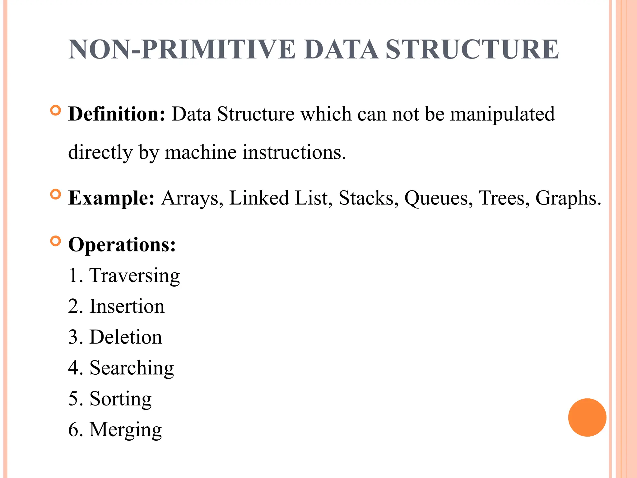
5.  Definition: Data Structure which can not be manipulated
directly by machine instructions.
 Example: Arrays, Linked List, Stacks, Queues, Trees, Graphs.
 Operations:
1. Traversing
2. Insertion
3. Deletion
4. Searching
5. Sorting
6. Merging
NON-PRIMITIVE DATA STRUCTURE

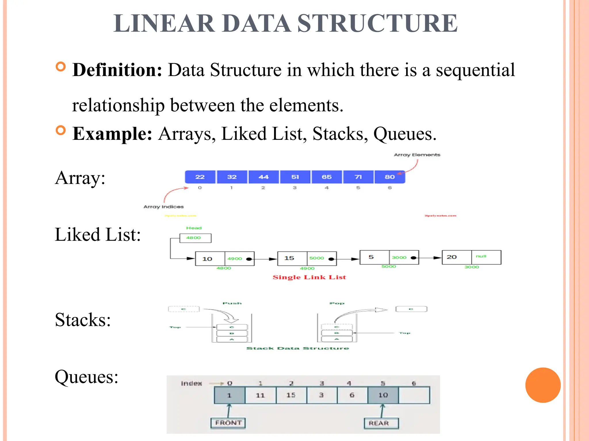
6.  Definition: Data Structure in which there is a sequential
relationship between the elements.
 Example: Arrays, Liked List, Stacks, Queues.
Array:
Liked List:
Stacks:
Queues:
LINEAR DATA STRUCTURE

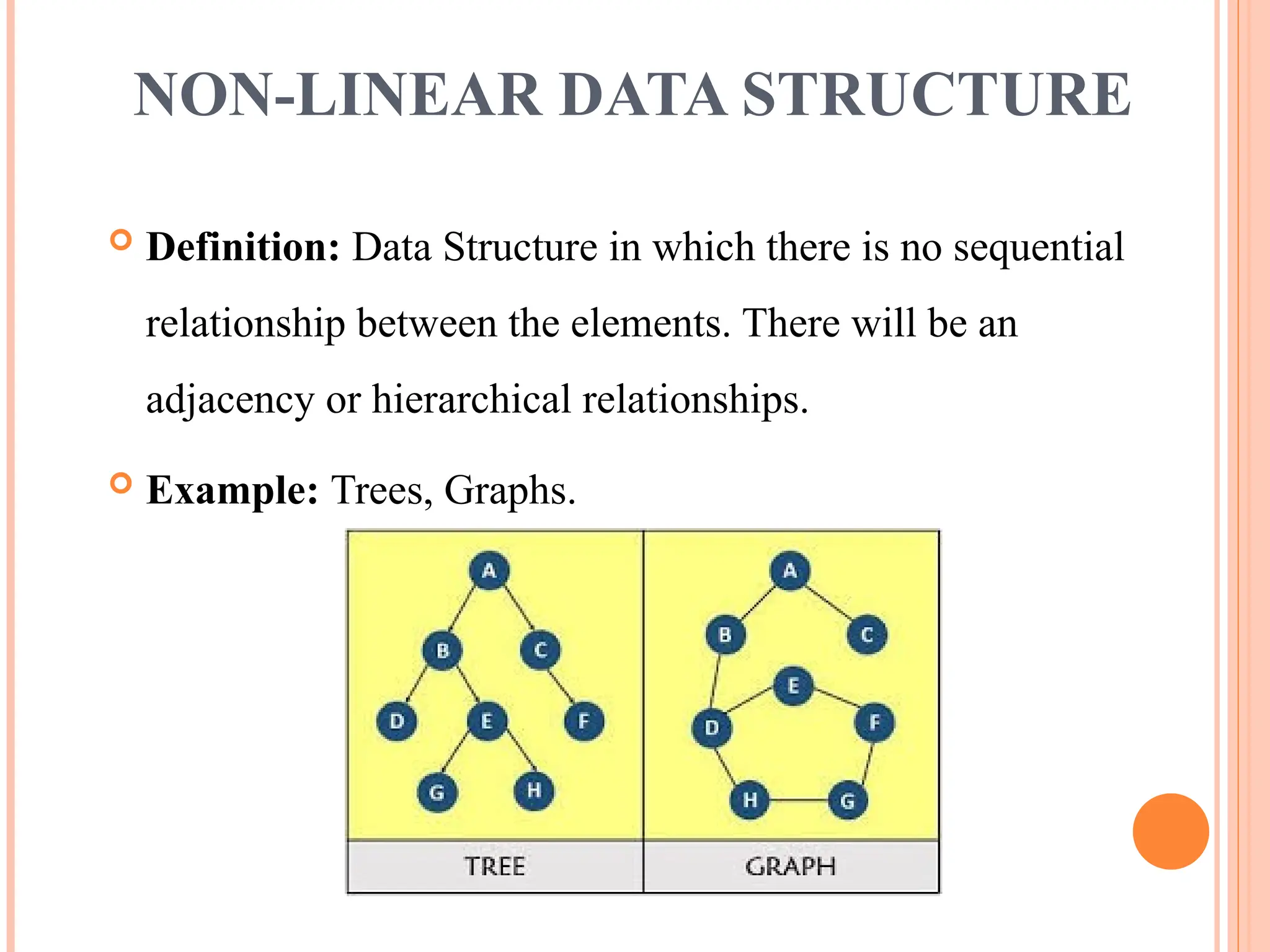
7.  Definition: Data Structure in which there is no sequential
relationship between the elements. There will be an
adjacency or hierarchical relationships.
 Example: Trees, Graphs.
NON-LINEAR DATA STRUCTURE

8. ARRAYS
 Definition: Collection of homogeneous elements with
only one name is called Arrays.
 Characteristics:
 Types:
1. One-Dimensional Array or Linear Array
2. Two-Dimensional Array
3. Multi-Dimensional Array

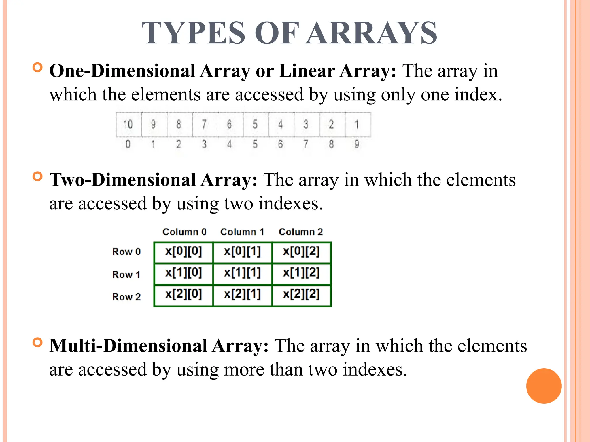
9. TYPES OF ARRAYS
 One-Dimensional Array or Linear Array: The array in
which the elements are accessed by using only one index.
 Two-Dimensional Array: The array in which the elements
are accessed by using two indexes.
 Multi-Dimensional Array: The array in which the elements
are accessed by using more than two indexes.

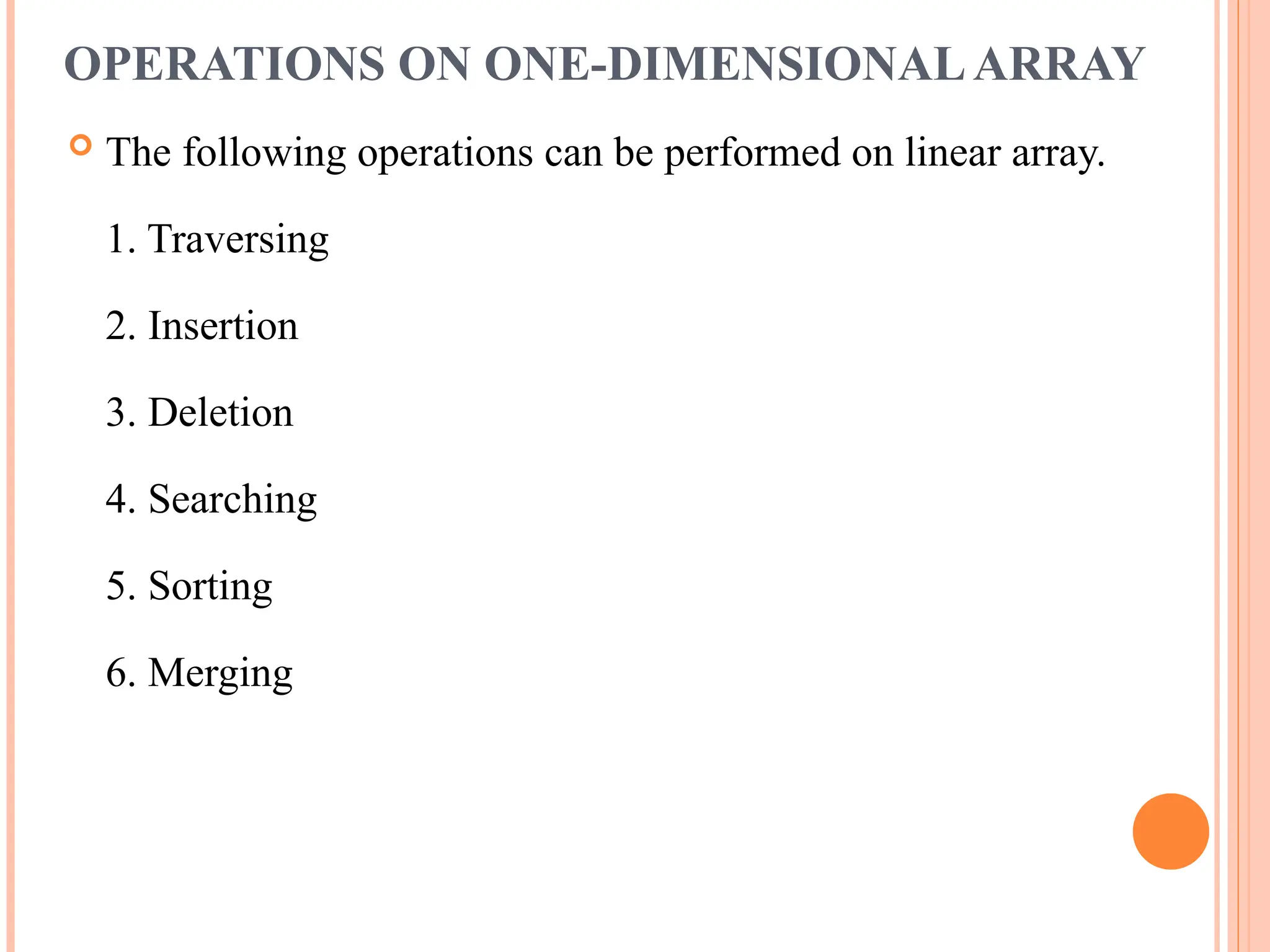
10. OPERATIONS ON ONE-DIMENSIONALARRAY
 The following operations can be performed on linear array.
1. Traversing
2. Insertion
3. Deletion
4. Searching
5. Sorting
6. Merging

11. TRAVERSING
 Traversal in a Linear Array is the process of
visiting each element once.
 Traversal is done by starting with the first
element of the array and reaching to the last.
 ALGORITHM:
TRAVERSAL(A, N)
Step1: FOR I = 0 to N-1
PROCESS(A[I])
[ end of FOR ]
Step2: Stop

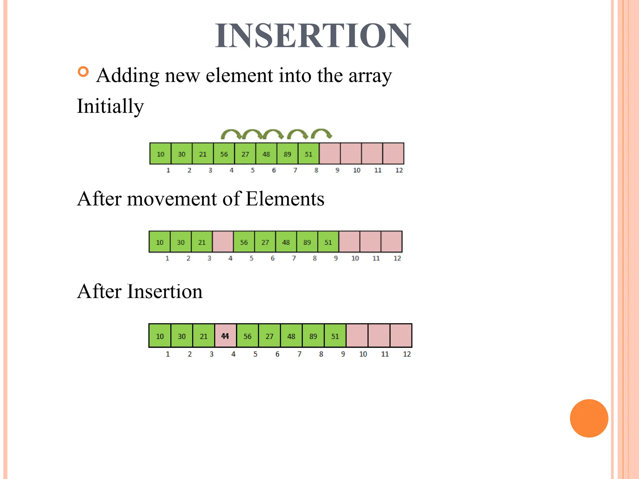
12. INSERTION
 Adding new element into the array
Initially
After movement of Elements
After Insertion

13. INSERTION
 ALGORITHM:
INSERTION(A, N, ELE, POS)
Step1: FOR I = N-1 DOWNTO POS
A[I+1] = A[I]
[end of FOR]
Step2: A[POS] = ELE
Step3: N = N + 1
Step4: Stop

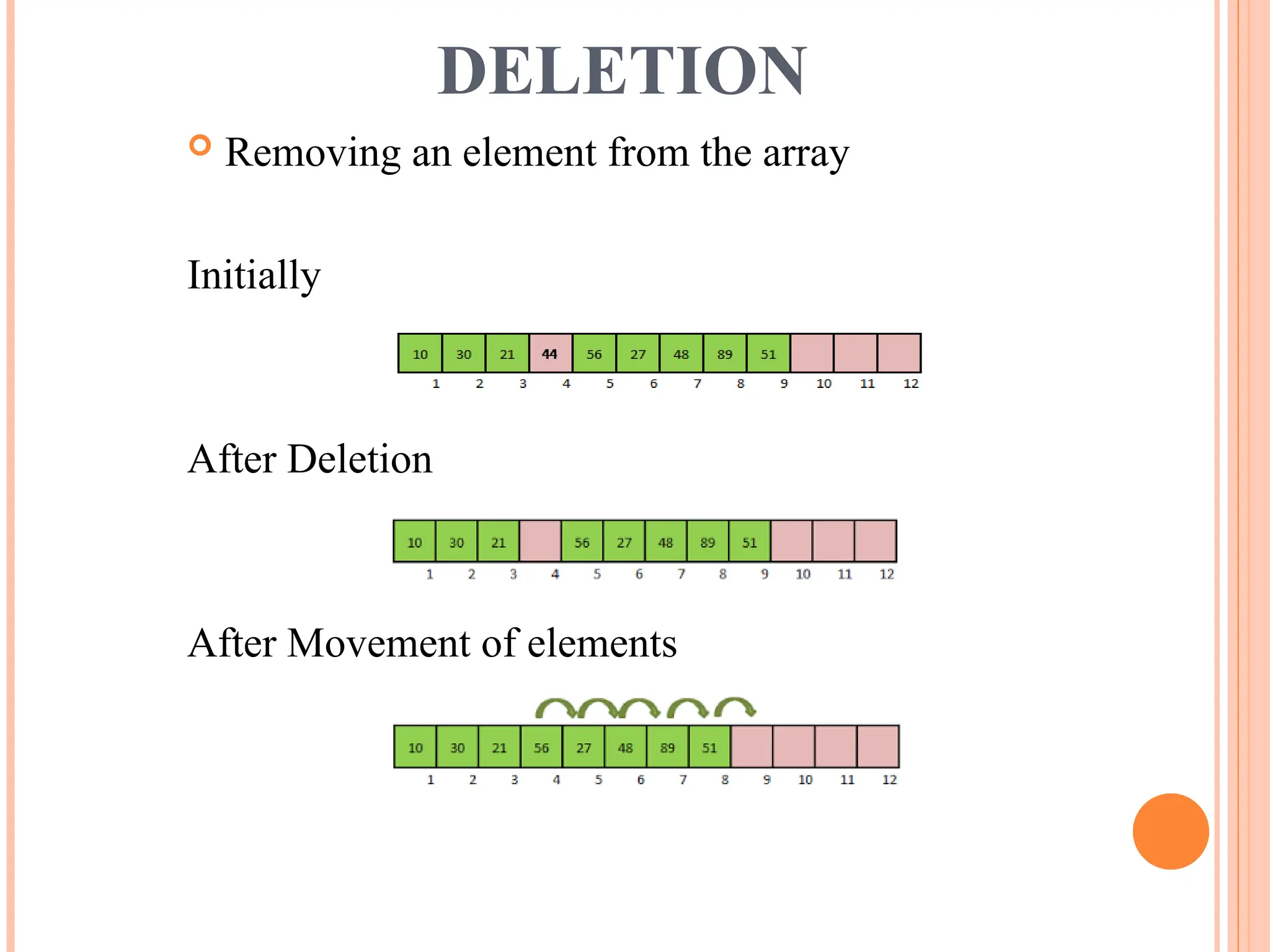
14. DELETION
 Removing an element from the array
Initially
After Deletion
After Movement of elements

15. DELETION
 ALGORITHM:
DELETION(A, N, ELE, POS)
Step1: ELE = A[POS]
Step2 FOR I = POS TO N – 2
A[I] = A[I+1]
[end of FOR]
Step3: N = N – 1
Step4: Stop

16. SEARCHING
 Definition: Checking weather the given
element is there in an array or not is called
Searching.
 Methods:
1. Linear Search or Sequential Search
2. Binary Search

17. LINEAR SEARCH
 It is also called Sequential Search.
 It can be applied on unsorted array.
 Algorithm:
LINEARSEARCH(A, N, KEY)
Step1: LOC = -1
Step2: FOR I = 1 TO N
IF (KEY == A[I])
LOC = I
goto Step3
[end of IF]
[end of FOR]
Step3: IF (LOC == – 1)
Print “ Element not found”
ELSE
Print “Element found at “, LOC
Step4: Stop

18. BINARY SEARCH
 It can be applied only on sorted array.
 It is based on Divide and Conquer Technique.
 Algorithm:
BINARYSEARCH(A, N, KEY)
Step1: LOC = -1, BEG = 0, END = N–1
Step2: Repeat WHILE (BEG <= END)
MID = (BEG + END)/2
IF ( KEY == A[MID] )
LOC = MID
goto Step3
ELSE IF (KEY < A[MID])
END = MID – 1
ELSE
BEG = MID + 1
[ end of IF ]
[ end of WHILE ]
Step3: IF (LOC == – 1)
Print “ Element not found”

19. BINARY SEARCH
Step3: IF (LOC == – 1)
Print “ Element not found”
ELSE
Print “Element found at “, LOC
[ end of IF ]
Step4: Stop

20. SORTING
 Definition: Arranging the elements in a
particular order is called sorting.
 Methods:
1. Bubble Sort
2. Selection Sort
3. Insertion Sort
4. Merge Sort
5. Quick Sort
6. Radix Sort
7. Heap Sort

21. BUBBLE SORT
 Algorithm:
BUBBLESORT(A, N)
Sept1. FOR I = 1 to N – 1
FOR J = 1 to N–I–1
IF ( A[J] > A[J+1]
TEMP = A[J]
A[J] = A[J+1]
A[J+1] = TEMP
[ end of IF ]
[ end of FOR ]
[ end of FOR ]

22. THANK YOU