Data Acquisition Techniques Using Pcs Second Edition 2nd Edition Howard Austerlitz

Data Acquisition Techniques Using Pcs Second
Edition 2nd Edition Howard Austerlitz download
https://ebookbell.com/product/data-acquisition-techniques-using-
pcs-second-edition-2nd-edition-howard-austerlitz-1642116
Explore and download more ebooks at ebookbell.com

Here are some recommended products that we believe you will be
interested in. You can click the link to download.
Mobile Forensics Cookbook Data Acquisition Extraction Recovery
Techniques And Investigations Using Modern Forensic Tools 1st Edition
Mikhaylov
https://ebookbell.com/product/mobile-forensics-cookbook-data-
acquisition-extraction-recovery-techniques-and-investigations-using-
modern-forensic-tools-1st-edition-mikhaylov-22009538
Analysis Techniques For Racecar Data Acquisition 2nd Edition Jorge
Segers
https://ebookbell.com/product/analysis-techniques-for-racecar-data-
acquisition-2nd-edition-jorge-segers-10922516
Towards Analytical Techniques For Optimizing Knowledge Acquisition
Processing Propagation And Use In Cyberinfrastructure And Big Data
Kreinovich
https://ebookbell.com/product/towards-analytical-techniques-for-
optimizing-knowledge-acquisition-processing-propagation-and-use-in-
cyberinfrastructure-and-big-data-kreinovich-6752720
Data Acquisition Systems From Fundamentals To Applied Design 1st
Edition Maurizio Di Paolo Emilio Auth
https://ebookbell.com/product/data-acquisition-systems-from-
fundamentals-to-applied-design-1st-edition-maurizio-di-paolo-emilio-
auth-4232050

Data Acquisition Using Labview Behzad Ehsani
https://ebookbell.com/product/data-acquisition-using-labview-behzad-
ehsani-5851398
Data Acquisition And Signal Processing For Smart Sensors Nikolay V
Kirianaki
https://ebookbell.com/product/data-acquisition-and-signal-processing-
for-smart-sensors-nikolay-v-kirianaki-1615050
Data Acquisition Handbook 3rd Edition Measurement Computing
Corporation
https://ebookbell.com/product/data-acquisition-handbook-3rd-edition-
measurement-computing-corporation-6781590
Advanced Data Acquisition And Intelligent Data Processing Vladimr
Haasz
https://ebookbell.com/product/advanced-data-acquisition-and-
intelligent-data-processing-vladimr-haasz-46517646
Phylogenomic Data Acquisition Principles And Practice W Bryan Jennings
https://ebookbell.com/product/phylogenomic-data-acquisition-
principles-and-practice-w-bryan-jennings-47604124

Data Acquisition
Tecliniques Using PCs
Second Edition

This Page Intentionally Left Blank

Data Acquisition
Tecliniques Using PCs
Second Edition
Howard Austerlitz
Parker Hannifin Corporation
Parl<er Aerospace
Electronic Systems Division
Smittitown, New Yorl<
ACADEMIC
PRESS
An imprint of Elsevier Science
Amsterdam Boston London New York Oxford Paris San Diego
San Francisco Singapore Sydney Tokyo

This book is printed on acid-free paper. ©
Copyright 2003, 1991, Elsevier Science (USA).
All rights reserved.
No part of this publication may be reproduced or transmitted in any form or by any means,
electronic or mechanical, including photocopy, recording, or any information storage and
retrieval system, without permission in writing from the publisher.
Requests for permission to make copies of any part of the work should be mailed to:
Permissions Department, Harcourt, Inc., 6277 Sea Harbor Drive, Orlando, Florida
32887-6777.
Academic Press
525 B Street, Suite 1900, San Diego, California 92101-4495, USA
http://www.academicpress.com
Academic Press
84 Theobald's Road, London WCIX 8RR, UK
http://www.academicpress.com
Library of Congress Control Number: 2002107710
International Standard Book Number: 0-12-068377-6
PRINTED IN THE UNITED STATES OF AMERICA
02 03 04 05 06 9 8 7 6 5 4 3 2 1

This book is dedicated to my wife, Kiel,
whose guidance and understanding
continue to make it all possible

Contents
Preface to the Second Edition xi
CHAPTER 1
Introduction to Data Acquisition
CHAPTER
Analog Signal Transducers.
2.1 Temperature Sensors 7
2.2 Optical Sensors 8
2.3 Force and Pressure Transducers 13
2.4 Magnetic Field Sensors 16
2.5 Ionizing Radiation Sensors 18
2.6 Position (Displacement) Sensors 19
2.7 Humidity Sensors 22
2.8 Fluid Flow Sensors 23
2.9 Fiber Optic Sensors 24
2.10 Other New Sensor Technologies 26
Analog Signal Conditioning
CHAPTER
3.1 Signal Conditioning Techniques 29
3.2 Analog Circuit Components 30
3.3 Analog Conditioning Circuits 37
VII

viii Contents
CHAPTER'
Analog/Digital Conversions
4.1 Digital Quantities 51
4.2 Data Conversion and DACs 55
4.3 ADCs 62
CHAPTER'
The PC
5.1 IBM PC/XT/AT and Compatible Computers 80
5.2 The IBM PC/XT 81
5.3 The IBM PC/AT 89
5.4 BIOS 93
5.5 PCI and Other Local Buses 95
5.6 PC Peripherals 102
CHAPTER I
Interfacing Hardware to a PC Bus
6.1 I/O Data Transfers 108
6.2 Memory Data Transfers 110
6.3 A Simple, 8-Bit I/O Port Design 111
6.4 DMA 115
6.5 Wait State Generation 115
6.6 Analog Input Card Design 117
6.7 16-Bit Data Transfers on ISA Computers 118
6.8 Plug and Play 120
6.9 Interfacing to the PCI Bus 121
Interfacing Software to the PC
7.1 DOS-Based PC Software Layers 123
7.2 Software Interrupts 125
7.3 Polled versus Interrupt-Driven Software 128
7.4 Special DOS Programs 132
7.5 DOS 133
7.6 Overcoming DOS Memory Limitations 135
7.7 Protected-Mode Operating Systems 137
CHAPTER

Contents ix
C
H
A
P
T
E
R 8
Standard Hardware Interfaces
8.1 Parallel versus Serial Digital Interfaces 142
8.2 Parallel Interfaces 144
8.3 Standard Serial Interfaces 163
8.4 PC Networks 184
CHAPTER
Data Storage and Compression Techniques
9.1 DOS Disk Structure and Files 191
9.2 Common DOS File Types 195
9.3 Windows File Systems 199
9.4 Data Compression Techniques 202
9.5 Commercial Data Compression Software 221
CHAPTER 10
Data Processing and Analysis
10.1 Numerical Representation 222
10.2 Data Analysis Techniques 229
CHAPTER 11
Commercial Data Acquisition Products
1L1 Commercial Data Acquisition Hardware Products 252
11.2 Commercial Data Acquisition Software Products 277
11.3 How to Choose Conmiercial Data Acquisition
Products 302
CHAPTER 12
Otiier PC Configurations and Hardware
for Data Acquisition
12.1 Alternative PC Architectures and Processors 304
12.2 Notebook PCs and PCMCIA Cards 312
12.3 Industrial and Embedded PCs 314
12.4 Image Capture Products 322

Contents
CHAPTER 13
Computer Programming Languages
13.1 Popular Programming Languages 330
13.2 Programming for Microsoft Windows 352
13.3 Considerations for Writing Computer Programs 357
CHAPTER 14
PC-Based Data Acquisition Applications
14.1 Ultrasonic Measurement System 362
14.2 Electrocardiogram Measurement System 369
14.3 Conmiercial Equipment Using Embedded PCs 374
14.4 Future Trends in PC-Based Data Acquisition 383
APPENDIX
Data Acquisition and Related
PC Product Manufacturers 385
Bibliography 401
Index 405

Preface to the _
Second Edition
Many things have changed in the decade since the first edition of Data
Acquisition Techniques Using PCs was pubUshed. PCs based on Intel micro-
processors and Microsoft Windows (the ubiquitous "Wintel" platform) have
become the dominant standard in small computers. They have also become
the most common computers in labs, offices, and industrial settings for data
acquisition and general-purpose applications. The world of PCs has continued
to evolve at a frenetic pace and the data acquisition market has changed along
with it, albeit more gradually (for example, ISA data acquisition cards are
still readily available).
Some of the changes in this edition include minimizing the amount of
material covering now-obsolete PCs (such as IBM's Micro Channel PS/2 line
and Apple's NuBus-based Macintosh line) while adding information about
more current standards (such as the PCI bus, the USB interface, and the Java
programming language). Most importantly, I have completely updated infor-
mation about commercially available data acquisition products (both hard-
ware and software) in Chapter 11. The listing of hardware and software data
acquisition product manufacturers in the Appendix is now twice the size it
was in the original edition.
This book is intended as a tutorial and reference for engineers, scientists,
students, and technicians interested in using a PC for data acquisition, anal-
ysis, and control applications. It is assumed that the reader knows the basic
workings of PCs and electronic hardware, although these aspects will be
briefly reviewed here. Several sources listed in the bibliography are good
introductions to many of these topics (both hardware and software).
This book stresses "real" applications and includes specific examples.
It is intended to provide all the information you need to use a PC as a data
acquisition system. In addition, it serves as a useful reference on PC technol-
ogy. Since the area of software is at least as important as hardware, if not
more so, software topics (such as programming languages, interfacing to a
PC's software environment, and data analysis techniques) are covered in detail.

xii Preface
I wish to acknowledge the help I received in writing this new edition.
My thanks to Academic Press for patiently seeing this project through. I am
grateful for the assistance I received from many manufacturers in the data
acquisition field, including Keithley Instruments, Laboratory Technologies,
and The Math Works. Finally, I want to acknowledge Omdorff, the laptop
editor, who kept me company during all those late nights at my PC.
Howard Austerlitz

C H A P T E R
Introduction t o -
Data Acquisition
Data acquisition, in the general sense, is the process of collecting information
from the real world. For most engineers and scientists these data are mostly
numerical and are usually collected, stored, and analyzed with a computer.
The use of a computer automates the data acquisition process, enabling the
collection of more data in less time with fewer errors. This book deals solely
with automated data acquisition and control using personal computers (PCs).
We will primarily concern ourselves with IBM-style PCs based on Intel
microprocessors (80x86 and Pentium families) running Microsoft operating
systems (MS-DOS and Windows). In general, the information in this book
is applicable to desktop, laptop, and embedded PCs. However, many plug-in
PCI data acquisition cards will also work in newer Apple Macintosh comput-
ers, with appropriate software drivers. In addition, USB, IEEE-1394 (FireWire)
and PCMCIA-based data acquisition hardware will work with any style of
computer which supports that interface, as long as software drivers are avail-
able for that platform.
An illustrative example of the utiUty of automated data acquisition is
measuring the temperature of a heated object versus time. Human observers are
limited in how fast they can record readings (say, every second, at best) and
how much data can be recorded before errors due to fatigue occur (perhaps after
5 minutes or 300 readings). An automated data acquisition system can easily
record readings for very small time intervals (i.e., much less than a millisecond),
continuing for arbitrarily long time periods (hmited mainly by the amount of
storage media available). In fact, it is easy to acquire too much data, which can
complicate the subsequent analysis. Once the data are stored in a computer,
they can be displayed graphically, analyzed, or otherwise manipulated.

2 CHAPTER 1 Introduction to Data Acquisition
Most real-world data are not in a form that can be directly recorded by
a computer. These quantities typically include temperature, pressure, distance,
velocity, mass, and energy output (such as optical, acoustic, and electrical
energy). Very often these quantities are measured versus time or position. A
physical quantity must first be converted to an electrical quantity (voltage,
current, or resistance) using a sensor or transducer. This enables it to be
conditioned by electronic instrumentation, which operates on analog signals
or waveforms (a signal or waveform is an electrical parameter, most often a
voltage, which varies with time). This analog signal is continuous and mono-
tonic, that is, its values can vary over a specified range (for example, some-
where between -5.0 volts and +3.2 volts) and they can change an arbitrarily
small amount within an arbitrarily small time interval.
To be recorded (and understood) by a computer, data must be in a digital
form. Digital waveforms have discrete values (only certain values are allowed)
and have a specified (usually constant) time interval between values. This
gives them a "stepped" (noncontinuous) appearance, as shown by the digitized
sawtooth in Figure 1-1. When this time interval becomes small enough, the
digital waveform becomes a good approximation to the analog waveform (for
example, music recorded digitally on a CD). If the transfer function of the
transducer and the analog instrumentation is known, the digital waveform can
be an accurate representation of the time-varying-quantity to be measured.
The process of converting an analog signal to a digital one is called
analog-to-digital conversion, and the device that does this is an analog-to-
digital converter (ADC). The resulting digital signal is usually an array of
digital values of known range (scale factor) separated by a fixed time interval
(or sampling interval). If the values are sampled at irregular time intervals,
the acquired data will contain both value and time information.
The reverse process of converting digital data to an analog signal is
called digital-to-analog conversion, and the device that does this is called a
(a) Analog Waveform (b) Digitized Waveform
Figure 1-1 Comparison of analog and digitized wavefornfis: (a) sawtooth analog
wavefornfi with (b) a coarse digitized representation.

Introduction to Data Acquisition
Keyboard Display Mass
Storage
Analog Inputs Analog Outputs
TTTTTITT
Inputs from Sensors Outputs to Controls
Figure 1-2 Simplified block diagram of a data acquisition system.
digital-to-analog converter (DAC). Some common applications for DACs
include control systems, waveform generation, and speech synthesis.
A general-purpose laboratory data acquisition system typically consists
of ADCs, DACs, and digital inputs and outputs. Figure 1-2 is a simplified
block diagram of such a system. Note that additional channels are often added
to an ADC via a multiplexer (or mux), used to select which one of the several
analog input signals to convert at any given time. This is an economical
approach when all the analog signals do not need to be simultaneously
monitored.
Economics is a major rationale behind using PCs for data acquisition
systems. The typical data acquisition system of 20-25 years ago, based on a
minicomputer, cost about 20 times as much as today's systems, based on PCs,
and ran at lower performance levels. This is largely due to the continuing
decrease in electronic component costs along with increased functionality
(more logic elements in the same package) and more sophisticated software.
The PC has become ubiquitous throughout our society, both in and out of
laboratories. Continuous improvements in hardware and software technologies
drive PCs and their peripheral devices to lower costs and higher performance.

CHAPTER 1 Introduction to Data Acquisition
Since PCs are commonplace in most labs and offices, the cost of imple-
menting a data acquisition system is often just the price of an add-in board
(or module) and support software, which is usually just a moderate expense.
For very simple applications, standard PC hardware (such as a sound card)
may be all you need for data acquisition.
There may be applications where a data acquisition system based on a
PC is not appropriate and a more expensive, dedicated system should be used.
The important system parameters for making such a decision include sam-
pling speed, accuracy, resolution, amount of data, multitasking capabilities,
and the required data processing and display. Of course, dedicated data
acquisition systems may be PC-based themselves, with an embedded PC (see
Chapter 12 for information on embedded PCs).
PC-based systems have fewer limitations in these areas than ever before,
even regarding sampling speed and handling large amounts of data. Newer,
high-performance PCs can even outperform some dedicated data acquisition
systems. The evolution of PCs based on the Intel 80x86 microprocessor (or
CPU), which includes the original IBM PC/XT/AT/PS2 computers, is dem-
onstrated in Table 1-1, showing processor speed, bus width, and the amount
of available memory space.
Apple's Macintosh computer line has also been used as a platform for
data acquisition. These machines, originally based on the Motorola 68000
family of microprocessors, had certain advantages over the older Intel-based
PCs, including a graphical, consistent operating environment and a linear
memory addressing space (the segmented addressing space of the Intel 80x86
family will be discussed in Chapter 5). Newer Macintosh computers use the
same PCI interface for add-in cards as contemporary Intel-based PCs (see
Chapter 5 for a discussion of the PCI bus).
TABLE 1-1
Intel 80x86 CPU Family Bus Size Characteristics
CPU
jsose
8088
i80286
180386
180486
1 Pentium
DATA BUS
WIDTH (bits)
16
8
16
32
32
32^^
ADDRESS BUS
WIDTH (bits)
20
20
24
32
32
32
MEMORY SPACE 1
(Mbytes)
1 1
1 1
16 1
4096 1
4096 1
4096 1
* Internal Bus = 64 bits wide.

Introduction to Data Acquisition 5
Software is as important to data acquisition systems as hardware capa-
bilities. Inefficient software can waste the usefulness of the most able data
acquisition hardware system. Conversely, well-written software can squeeze
the maximum performance out of mediocre hardware. Software selection is
at least as important as hardware selection and often more complex.
Data acquisition software controls not only the collection of data, but
also its analysis and eventual display. Ease of data analysis and presentation
are the major reasons behind using computers for data acquisition in the first
place. With the appropriate software, computers can process the acquired data
and produce outputs in the form of tables or plots. Without these capabilities,
you are not doing much more than using a sophisticated (and expensive) data
recorder.
An additional area of software use is that of control. Computer outputs
may control some aspects of the system that is being measured, as in auto-
mated industrial process controls. The software must be able to measure
system parameters, make decisions based on those measurements, and vary
the computer outputs accordingly. For example, in a temperature regulation
system, the input would be a temperature sensor and the output would control
a heater. In control applications, software reliability and response time are
paramount. Slow or erroneous software responses could cause physical dam-
age. Control applications are especially important for embedded PCs, which
package full PC functionality into a small form factor, such as PC-104 (see
Chapter 12).
A recent, important software capability is Internet access. Many new
products allow you to perform remote data acquisition using the Internet (and
its TCP/IP protocol). It is now fairly simple to monitor and control a data
acquisition system located nearly anywhere in the world as well as share the
data with a large group of colleagues.
There is a plethora of PC-based software packages commercially avail-
able, which can collect, analyze, and display data graphically, using little or
no programming (see Chapter 11). They allow users to concentrate on their
applications, instead of worrying about the mechanics of getting data from
point A to point B, or how to plot a set of Cartesian coordinates. Many
commercial software packages contain all three capabilities of data acquisi-
tion, analysis, and display (the so-called "integrated" packages), whereas
others are optimized for only one or two of these areas.
The important point is that you do not have to be a computer expert or
even a programmer to implement an entire PC-based data acquisition system.
Best of all, you do not have to be rich, either.
The next chapter examines the world of analog signals and their trans-
ducers, the "front end" of any data acquisition system.

C H A P T E R
Analog Signal
Transducers
Most real-world events and their measurements are analog. That is, the mea-
surements can take on a wide, nearly continuous range of values. The physical
quantities of interest can be as diverse as heat, pressure, light, force, velocity,
or position. To be measured using an electronic data acquisition system, these
quantities must first be converted to electrical quantities such as voltage,
current, or impedance.
A transducer converts one physical quantity into another. For the pur-
poses of this book, all the transducers mentioned convert physical quantities
into electrical ones, for use with electronic instrumentation. The mathematical
description of what a transducer does is its transfer function, often designated
H. So the operation of a transducer can be described as
Output Quantity = Hx Input Quantity
Since the transducer is the "front end" of the data acquisition system,
its properties are critical to the overall system performance. Some of these
properties are sensitivity (the efficiency of the energy conversion), stability
(output drift with a constant input), noise, dynamic range, and linearity. Very
often the transfer function is dependent on the input quantity. It may be a
linear function for one range of input values and then become nonlinear for
another range (such as a square-law curve). Looking at sensitivity and noise,
if the transducer's sensitivity is too low, or its noise level too high, signal
conditioning may not produce an adequate signal-to-noise ratio.
Often the transducer is the last consideration in a data acquisition
system, since it is seen as mundane. Yet, it should be the primary consideration.

2.1 Temperature Sensors 7
The characteristics of the transducer, in large part, determine the Umits of a
system's performance.
Now we will look at some common transducers in detail.
2.1 Temperature Sensors.
Temperature sensors have electrical parameters that vary with temperature,
following well-characterized transfer functions. In fact, nearly all electronic
components have properties which vary with temperature. Many of them
could potentially be temperature transducers if their transfer functions were
well behaved and insensitive to other variables.
2.1.1 Thermocouples
The thermocouple converts temperature to a small DC voltage or current. It
consists of two dissimilar metal wires in intimate contact in two or more
junctions. The output voltage varies linearly with the temperature difference
between the junctions—the higher the temperature difference, the higher the
voltage output. This linearity is a chief advantage of using a thermocouple, as
well as its ruggedness as a sensor. In addition, thermocouples operate over very
large temperature ranges and at very high temperatures (some, over 1000°C).
Disadvantages include low output voltage (especially at lower tempera-
tures), low sensitivity (typical output voltages vary only about 5 mV for a 100°C
temperature change), susceptibility to noise (both externally induced and inter-
nally caused by wire imperfections and impurities), and the need for a reference
junction (at a known temperature) for calibration. Most data acquisition hard-
ware designed for temperature measurements contain an electronic reference
junction. You must enter the thermocouple material type you are using, so it is
properly calibrated. Common thermocouple materials include copper/constan-
tan (Type T), iron/constantan (Type J), and chromel/alumel (Type K).
When several thermocouples, made of the same materials are combined
in series, they are called a thermopile. The output voltage of a thermopile consists
of the sum of all the individual thermocouple outputs, resulting in increased
sensitivity. All the reference junctions are kept at the same temperature.
2.1.2 Thermistors
A thermistor is a temperature-sensitive resistor with a large, nonlinear, negative
temperature coefficient. That is, its resistance decreases nonlinearly as temper-
ature increases. It is usually composed of a mixture of semiconductor materials.

8 CHAPTER 2 Analog Signal Transducers
It is a very sensitive device, but has to be properly calibrated for the desired
temperature ranges, since it is a nonlinear detector. Repeatability from device
to device is not very good. Over relatively small temperature ranges it can
approximate a linear response. It is prone to self-heating errors due to the
power dissipated in it (P = IR), This effect is minimized by keeping the
current passing through the thermistor to a minimum.
2.1.3 Resistance Temperature Detectors
Resistance temperature detectors (RTDs) rely on the temperature dependence
of a material's electrical resistance. They are usually made of a pure metal
having a small but accurate positive temperature coefficient. The most accu-
rate RTDs are made of platinum wire and are well characterized and linear
from 14°K to higher than 600°C.
2.1.4 Monolithic Temperature Transducers
The monolithic temperature transducer is a semiconductor temperature sensor
combined with all the required signal conditioning circuitry and located in
one integrated circuit. This device typically produces an output voltage pro-
portional to the absolute temperature, with very good accuracy and sensitivity
(a typical device produces an output of 10 mV per degree Kelvin over a
temperature range of 0-100 degrees Celsius). The output of this device can
usually go directly into an ADC with very little signal conditioning.
2.2 Optical Sensors
Optical sensors are used for detecting light intensity. Typically, they respond
only to particular wavelengths or spectral bands. One sensor may respond
only to visible light in the blue-green region, while another sensor may have
a peak sensitivity to near-infrared radiation.
2.2.1 Vacuum Tube Photosensors
This class of transducers consists of special-purpose vacuum tubes used as
optical detectors. They are all relatively large, require a high-voltage power
supply to operate, and are used only in very specialized applications (as is
true with vacuum tubes in general). These sensors exploit the photoelectric
effect, when photons of light striking a suitable surface produce free electrons.

Incident
Photons
Figure 2-1 Vacuum photodiode.
The vacuum photodiode consists of a photocathode and anode in a
glass or quartz tube. The photocathode emits electrons when struck by
photons of light. These electrons are accelerated to the anode by the high (+)
voltage and produce a current pulse in the external load resistor /?L (see Figure
2-1). These tubes have relatively low sensitivity, but they can detect high-
frequency light variations or modulation (as high as 100 MHz to 1 GHz), for
an extremely fast response.
The gas photodiode is similar to a vacuum photodiode, except the tube
contains a neutral gas. A single photoelectron (emitted by the photocathode)
can collide with several gas atoms, ionizing them and producing several extra
electrons. So, more than one electron reaches the anode for every photon.
This gas amplification factor is usually 3-5 (larger values cause instabilities).
These tubes have a limited frequency response of less than 10 kHz, resulting
in a much slower response time.
Thephotomultiplier tube (PMT) is the most popular vacuum tube device
in this category. It is similar to a vacuum photodiode with several extra
electrodes between the photocathode and anode, called dynodes. Each dynode
is held at a more positive voltage than the previous dynode (and the cathode)
via a resistor voltage-divider network (see Figure 2-2). Photoelectrons emitted
by the photocathode strike the first dynode, which emits several secondary
electrons for each photoelectron, amplifying the photoelectric effect. These
secondary electrons strike the next dynode and release more electrons. This
process continues until the electrons reach the end of the dynode amplifier
chain. There, the anode collects all the electrons produced by a single photon,
resulting in a relatively large current pulse in the external circuit.

Dynode
Dynode
Dynode
Incident
Anode Cathode Photon
(a) Cross section of typical PMT
Anode
^Dynode
* Dynode
* Dynode
* Dynode
»Dynode
»DynodeI
^Cathode!
(b) Wiring diagrann for typical PMT
Figure 2-2 Photomultiplier tube (PMT).
The PMT exhibits very high gain, in the range of 10-10 electrons
emitted per incident photon. This is determined by the number of dynodes,
the photocathode sensitivity, power supply voltage, and tube design factors.
Some PMTs can detect individual photons!
A PMT's output pulses can be measured as a time-averaged current
(good for detecting relatively high light levels) or in an individual pulse-
counting mode (good for very low light levels) measuring the number of
pulses per second. Then, a threshold level is used tofilterout unwanted pulses
(noise) below a selected amplitude.
Some of the noise produced in a PMT is spontaneous emission from
the electrodes, which occurs even in the absence of light. This is called the
dark count, which determines the PMT's sensitivity threshold. So, the number
of photons striking the PMT per unit time must be greater than the dark count
for the photons to be detected. In addition, most PMTs have a fairly low
quantum efficiency, a measure of how many photons are required to produce
a measurable output (expressed as a percentage, where 100% means that

every photon striking the sensor will produce an output). Also, PMTs have
a limited usable life, as the photocathode wears out with time.
2.2.2 Photoconductive Cells
A photoconductive cell consists of a thin layer of material, such as cadmium
sulfide (CdS) or cadmium selenide (CdSe) sandwiched between two elec-
trodes, with a transparent window. The resistance of a cell decreases as the
incident light intensity increases. These cells can be used with any resistance-
measuring apparatus, such as a bridge. They are commonly used in photo-
graphic light meters. A photoconductive cell is usually classified by maximum
(dark) resistance, minimum (light) resistance, spectral response, maximum
power dissipation, and response time (or frequency).
These devices are usually nonlinear and have aging and repeatability
problems. They exhibit hysteresis in their response to light. For example, the
same cell exposed to the same light source may have a different resistance,
depending on the light levels it was previously exposed to.
2.2.3 Photovoltaic (Solar) Cells
These sensors are similar in construction to photoconductive cells. They are
made of a semiconductor material, usually silicon (Si) or gallium arsenide
(GaAs), that produces a voltage when exposed to light (of suitable wavelength).
They require no external power supply and very large cells can be used as DC
power sources. They have a relatively slow response time to light variations
but are fairly sensitive. Since the material used must be grown as a single
crystal, large photovoltaic cells are very expensive.
A large amount of research has been conducted in recent years in an
attempt to produce less expensive photovoltaic cells made from either amor-
phous, polycrystalline, or thin-film semiconductors. If these low-cost devices
can attain light conversion efficiency similar to that of monocrystalline cells
(in the range of 15-20%), they can become a practical source of electric energy.
2.2.4 Semiconductor Light Sensors
The members of this class of transducers are all based on a semiconductor
device, such as a diode or transistor, whose output current is a function of
the light (of suitable wavelength) incident upon it.
The photodiode is a PN junction diode with a transparent window that
produces charge carriers (holes and electrons) at a rate proportional to the
incident light intensity. So the photodiode acts as a photoconductive device,
varying the current in its external circuit (but, being a semiconductor, it does
not obey Ohm's law). A photodiode is a versatile device with a high frequency

response and a linear output, but low sensitivity, and it usually requires large
amounts of amplification. It typically uses a transconductance amplifier,
which converts the photodiode output current to a voltage. A common pho-
todiode sensor is the PIN diode, which has an insulating region between the
p and n materials. This device usually requires a reverse DC bias voltage for
optimum performance (speed and sensitivity). Conventional silicon photo-
diodes have usable sensitivity to light wavelengths in the range of 450-1050
nanometers (from the visible spectrum into the near infrared). For longer
wavelengths, other semiconductors, such as indium gallium arsenide
(InGaAs) are used.
The phototransistor is similar to a photodiode, except that the transistor
can provide amplification of the PN junction's light-dependent current. The
transistor's emitter-base junction is the light-sensitive element. A photodar-
lington is a special phototransistor, composed of two transistors in a high-gain
circuit. The phototransistor offers much higher sensitivity than the photodiode
at the expense of a much lower bandwidth (response time) and poorer linearity.
The avalanche photodiode (APD) is a special photodiode which has
internal gain and is a semiconductor analog to the PMT. This gain is normally
in the range of 10 to a few hundred (typically around 100 for a silicon device).
The APD employs a high reverse bias (from several hundred volts up to a
few thousand volts) to produce a strong internal electricalfieldthat accelerates
the electrons generated by the incident photons and results in secondary
electrons from impact ionization. This is the electron avalanche, resulting in
gain. Advantages of the APD are small size, solid-state reliability (as long as
the breakdown voltage is not exceeded), high quantum efficiency, and a large
dynamic range. Compared to PMTs, APDs have much lower gain, smaller
light-collecting areas, and a high temperature sensitivity. APD bias must be
temperature compensated to keep gain constant.
The charge-coupled device (CCD) is a special optical sensor consisting
of an array (one- or two-dimensional) of light-sensitive elements. When photons
strike a photosensitive area, electron/hole pairs are created in the semiconductor
crystal. The holes move into the substrate and the electrons remain in the
elements, producing a net electrical charge. The amount of charge is propor-
tional to the amplitude of incident light and the exposure time. The charge at
each photosensitive element is then read out serially, via support electronics.
CCDs are conmionly used in many imaging systems, including video cameras.
2.2.5 Thermoelectric Optical Sensors
This class of transducers convert incident light to heat and produce a tem-
perature output dependent on light intensity, by absorbing all the incident
radiation in a "black box." They generally respond to a very broad light

spectrum and are relatively insensitive to wavelength, unlike vacuum tube
and solid-state sensors. However, they have very slow response times and
low sensitivities and are best suited for measuring static or slowly changing
light levels, such as calibrating the output of a light source.
The bolometer varies its resistance with thermal energy produced by
incident radiation. The most common detector element used in a bolometer
is a thermistor. They are also commonly used for measuring microwave power
levels.
The thermopile, as discussed under temperature sensors, is more com-
monly used than individual thermocouples in light-detecting applications
because of its higher sensitivity. It is often used in infrared detectors.
2.3 Force and Pressure Transducers
A wide range of sensors are used for measuring force and pressure. Most
pressure transducers rely on the movement of a diaphragm mounted across
a pressure differential. The transducer measures this minute movement.
Capacitive and inductive pressure sensors operate the same way as capacitive
and inductive displacement sensors, which are described later on.
2.3.1 strain Gages
Strain gages are transducers used for directly measuring forces and their
resulting strain on an object. Stress on an object produces a mechanical
deformation—strain—defined as
Strain = length change/length
Strain gages are conductors (often metallic) whose resistance varies with strain.
For example, as a wire is stretched, its resistance increases. Strain gages are
bonded to the object under stress and are subject to the same forces. They are
very sensitive to strain in one direction only (the axis of the conductor).
A simple unbonded strain gage consists of free wires on supports
bonded to the stressed surface. These are not usually used (outside of labo-
ratory demonstrations) because of their large size and mechanical clumsiness.
The bonded strain gage overcomes these problems by putting a zigzag
pattern of the conductor on an insulating surface, as shown in Figure 2-3.
These are relatively small, have good sensitivity, and are easily bonded to the
surface under test. The conductor in a bonded strain gage is a metallic wire,
foil, or thin film.

SENSITIVE AXIS
Figure 2-3 Sinfipie, one-dimensional strain gage.
Strain gage materials must have certain, well-controlled properties. The
most important is sensitivity or gage factor (GF), which is the change in
resistance per change in length. Most metallic strain gages have a GF in the
range of 2 to 6. The material must also have a low temperature coefficient of
resistance as well as stable elastic properties and high tensile strength. Often,
strain gages are subject to very large stresses as well as wide temperature swings.
Semiconductor strain gages, usually made of silicon, have a much
higher GF than metals (typically in the range of 50 to 200). However, they
also have much higher temperature coefficients, which have to be compen-
sated for. They are conmionly used in monolithic pressure sensors.
Because of their relatively low sensitivities (resistance changes nomi-
nally 0.1 to 1.0%), strain gages require bridge circuits to produce useful
outputs. (We will discuss bridge circuits in Chapter 3.) If a second, identical
strain gage, not under stress, is put into the bridge circuit, it acts as a
temperature compensator.
2.3.2 Piezoelectric Transducers
Piezoelectric transducers are used for, among other things, measuring time-
varying forces and pressures. They do not work for static measurement, since
they produce no output from a constant force or pressure.
Certain crystalline materials (including quartz, barium titanate, and
lithium niobate) generate an electromotive force (emf) when mechanically
stressed. Conversely, when a voltage is applied to the crystal, it will become
mechanically distorted. This is the piezoelectric effect.
If electrodes are placed on suitable (usually opposite) faces of the crystal,
the direction of the deforming force can be controlled. If an AC voltage is
applied to the electrodes, the crystal can produce periodic motion, resulting

Electrodes
Ultrasonic ^
Waves N
Crystal
/
/
^ ^
- < ^
Electrodes
K Ultrasonic
y^ Waves
Ultrasonic
Waves
i
Sr
Ultrasonic
Waves
^
Crystal
^ — • ^ ^ — ^
(a) Longitudinal Mode (b) Transverse Mode
Figure 2-4 Oscillation modes of piezoelectric crystals.
in an acoustic wave, which can be transmitted through other material. When
an acoustic wave strikes a piezoelectric crystal, it produces an AC voltage.
When a piezoelectric crystal oscillates in the thickness or longitudinal
mode, an acoustic wave is produced, where the direction of displacement is
the direction of wave propagation, as shown in Figure 2-4a. When the crystal's
thickness equals a half-wavelength of the longitudinal wave's frequency (or
an odd multiple half-wavelength) it is resonant at that frequency. At resonance
its mechanical motion is maximum along with the acoustic wave output. And
when it is detecting acoustic energy, the output voltage is maximum for the
resonant frequency.
This characteristic is applied to quartz crystal oscillators, used as highly
accurate electronic frequency references in a broad range of equipment, from
computers to digital watches.
Typically, piezoelectric crystals are used as ultrasonic transducers for
frequencies above 20 kHz, up to about 100 MHz. The limitation on frequency
range is due to the impracticalities of producing crystals thin enough for very
high frequencies, or the unnecessary expense of producing very thick crystals
for low frequencies (where electromagnetic transducers work better).

Other crystal deformation modes are transverse, where the direction of
motion is at right angles to the direction of wave propagation (as shown in
Figure 2-4b), and shear, which is a mix of longitudinal and transverse modes.
These modes all have different resonant frequencies.
Piezoelectric transducers have a wide range of applications, besides
dynamic pressure and force sensing, including the following:
1. Acoustic microscopy for medical and industrial applications, such
as "seeing" through materials that are optically opaque. An example
is the sonogram.
2. Distance measurements including sonar and range finders.
3. Sound and noise detection such as microphones and loudspeakers
for audio and ultrasonic acoustic frequencies.
2.4 Magnetic Field Sensors
This group of transducers is used to measure either varying or fixed magnetic
fields.
2.4.1 Varying Magnetic Field Sensors
These transducers are simple inductors (coils) that can measure time-varying
magnetic fields such as those produced from an AC current source. The
magnetic flux through the coil changes with time, so an AC voltage is induced
that is proportional to the magnetic field strength.
These devices are often used to measure an alternating current (which
is proportional to the AC magnetic field). For standard 60-Hz loads, trans-
formers are used that clamp around a conductor (no direct electrical contact).
These are usually low-sensitivity devices, good for 60 Hz currents greater
than 0.1 ampere.
2.4.2 Fixed Magnetic Field Sensors
Several types of transducers are commonly used to measure static and slowly
varying magnetic fields, such as those produced by a permanent magnet or
a DC electromagnet.
Hall Effect Sensors When a current-carrying conductor strip is placed with
its plane perpendicular to an applied magnetic field (B) and a control current
(IQ) is passing through it, a voltage (VH) is developed across the strip at right

2.4 Magnetic Field Sensors 17
Current
Source
•cl
Magnetic Field
/ ^ 1 ^
r^>^
^^ ^
i
^ ^ ^ s . ^ ^
/^^5s^ • ^ ^
vSl
Figure 2-5 Hall effect nfiagnetic field sensor.
angles to 1Q and B, as shown in Figure 2-5. VH is known as the Hall voltage
and this is the Hall effect:
VH = Kl^BId
where:
B = magnetic field (in gauss),
d = thickness of strip,
K = Hall coefficient.
The value of K is very small for most metals, but relatively large for certain
n-type semiconductors, including germanium, silicon, and indium arsenide.
Typical outputs are still just a few millivolts/kilogauss at rated /c- Although
a larger IQ or a smaller d should increase V, these would cause excessive self-
heating of the device (by increasing its resistance) and would change its
characteristics as well as lower its sensitivity. The resistance of typical Hall
devices varies from a few ohms to hundreds of ohms.
SQUIDs SQUID stands for superconducting quantum interference device, a
superconducting transducer based on the Josephson junction. A SQUID is a
thin-film device operating at liquid helium temperature (~4°K), usually made
from lead or niobium. The advent of higher temperature superconductors that

can operate in the liquid nitrogen region (~78°K) may produce more practical
and inexpensive SQUIDs.
A SQUID element is a Josephson junction that is based on quantum
mechanical tunneling between two superconductors. Normally, the device is
superconducting, with zero resistance, until an applied magnetic field switches
it into a normal conducting state, with some resistance. If an external current
is applied to the device (and it must be low enough to prevent the current
from switching it to a normal conductive state—another Josephson junction
property), the voltage across the SQUID element switches between zero and
a small value. The resistance and measured voltage go up by steps (or quanta)
as the applied magnetic field increases. It measures very small, discrete
(quantum) changes in magnetic field strength.
Practical SQUIDs are composed of arrays of these individual junctions
and are extremely sensitive magnetometers. For example, they are used to
measure small variations in the earth's magnetic field, or even magnetic fields
generated inside a living brain.
2.5 Ionizing Radiation Sensors.
Ionizing radiation can be particles produced by radioactive decay, such as
alpha or beta radiation, or high-energy electromagnetic radiation, including
gamma and X-rays. In many of these detectors, a radiation particle (a photon)
collides with an active surface material and produces charged particles, ions,
and electrons, which are then collected and counted as pulses (or events) per
second or measured as an average current.
2.5.1 Geiger Counters
When the electric field strength (or voltage) is high enough in a gas-filled
tube, electrons produced by primary ionization gain enough energy between
coUisions to produce secondary ionization and act as charge multipUers. In
a Geiger-Muller tube the probability of this secondary ionization approaches
unity, producing an avalanche effect. So, a very large current pulse is caused
by one or very few ionizing particles. The Geiger-Muller tube is made of
metal and filled with low-pressure gas (at about 0.1 atm) with a fine, electri-
cally isolated wire running through its center, as shown in Figure 2-6.
A Geiger counter requires a recovery time (dead time) of -200 micro-
seconds before it can produce another discharge (to allow the ionized particles
to neutralize). This limits its counting rate to less than a few kilohertz.

Fine Wire
Glass Seal ^ _
Brass Tube
High-Voltage
Power Supply
Gas Pressure ~ 0.1 Atm
Glass Seal
Figure 2-6 Typical Geiger-Muller tube.
2.5.2 Semiconductor Radiation Detectors
Some/7-n junction devices (typically diodes), when properly biased, can act
as solid-state analogs of an ion chamber, where a high DC voltage across a
gas-filled chamber produces a current proportional to the number of ionizing
particles striking it per unit time, due to primary ionization. When struck by
radiation the devices produce charge carriers (electrons and holes) as opposed
to ionized particles. The more sensitive (and useful) devices must be cooled
to low temperatures (usually 78°K, by liquid nitrogen).
2.5.3 Scintillation Counters
This device consists of afluorescentmaterial that emits Ught when struck by a
charged particle or radiation, similar to the action of a photocathode in a pho-
todiode. The emitted hght is then detected by an optical sensor, such as a PMT.
2.6 Position (Displacement) Sensors
A wide variety of transducers are used to measure mechanical displacement
or the position of an object. Some require actual contact with the measured
object; others do not.

2.6.1 Potentiometers
The potentiometer (variable resistor) is often mechanically coupled for dis-
placement measurements. It can be driven by either AC or DC signals and
does not usually require an amplifier. It is inexpensive but cannot usually be
used in high-speed applications. It has limited accuracy, repeatability, and
lifetime, due to mechanical wear of the active resistive material. These devices
can either be conventional rotary potentiometers or have a linear configuration
with a slide mechanism. Often, the resistive element is polymer-based to
increase its usable life.
2.6.2 Capacitive and Inductive Sensors
Simple capacitive and inductive sensors produce a change in reactance
(capacitance or inductance) with varying distance between the sensor and the
measured object. They require AC signals and conditioning circuitry and have
limited dynamic range and linearity. They are typically used over short dis-
tances as a proximity sensor, to determine if an object is present or not. They
do not require contact with the measured object.
2.6.3 LVDTs
The LVDT {linear voltage differential transformer) is a versatile device used
to measure displacement. It is an inductor consisting of three coils wound
around a movable core, connected to a shaft, as shown in Figure 2-7. The
center coil is the transformer's primary winding. The two outer coils are
connected in series to produce the secondary winding. The primary is driven
by an AC voltage, typically between 60 Hz and several kilohertz. At the null
point (zero displacement), the core is exactly centered under the coils and
the secondary output voltage is zero. If the shaft moves, and the core along
with it, the output voltage increases linearly with displacement, as the induc-
tive coupling to the secondary coils becomes unbalanced. A movement to
one side of the null produces a 0° phase shift between output and input signal.
A movement to the other side of null produces a 180° phase shift.
If the displacement is kept within a specified range, the output voltage
varies linearly with displacement. The main disadvantages to using an LVDT
are its size, its complex control circuitry, and its relatively high cost.
2.6.4 Optical Encoders
The optical encoder is a transducer commonly used for measuring rotational
motion. It consists of a shaft connected to a circular disc, containing one or
more tracks of alternating transparent and opaque areas. A light source and

Secondary Coil 1 Primary Coil Secondary Coil 2
Core
Shaft
(a) Cross-Section View
- Signal Output -
Secondary Coil 1
uuuu
Core
Secondary Coil 2
uuuu
nnnn
Primary Coil
AC Input •
(b) Schematic Diagram
Figure 2-7 Linear variable differential transfornfier (LVDT).
an optical sensor are mounted on opposite sides of each track. As the shaft
rotates, the Ught sensor emits a series of pulses as the light source is inter-
rupted by the pattern on the disc. This output signal can be directly compatible
with digital circuitry. The number of output pulses per rotation of the disc is
a known quantity, so the number of output pulses per second can be directly
converted to the rotational speed (or rotations per second) of the shaft. Encod-
ers are commonly used in motor speed control applications. Figure 2-8 shows
a simple, one-track encoder wheel.
An incremental optical encoder has two tracks, 90° out of phase with
each other, producing two outputs. The relative phase between the two chan-
nels indicates whether the encoder is rotating clockwise or counterclockwise.
Often there is a third track that produces a single index pulse, to indicate an
absolute position reference. Otherwise, an incremental encoder produces only
relative position information. The interface circuitry or computer must keep
track of the absolute position.

Figure 2-8 Simple one-track optical encoder wheel (24 lines = 15° resolution).
An absolute optical encoder has several tracks, with different patterns on
each, to produce a binary code output that is unique for each encoded position.
There is a track for each output bit, so an 8-bit absolute encoder has 8 tracks,
8 outputs and 256 output combinations, for a resolution of 360/256 = 1.4°. The
encoding is not always a simple binary counting pattern, since this would
result in adjacent counts where many bits change at once, increasing the
likelihood of noise and reading errors. A Gray code is often used, because
it produces a pattern where each adjacent count results in only one bit
change. An absolute encoder is usually much more expensive than a compa-
rable incremental encoder. Its main advantage is the ability to retain absolute
position information, even when system power is removed.
2.6.5 Ultrasonic Range Finder
In Chapter 14, an ultrasonic range finder is discussed, as a noncontact dis-
placement measurement technique. The time it takes an ultrasonic pulse to
reflect from an object is measured and the distance to the object calculated
from that time delay, using a known ultrasonic velocity.
2.7 Humidity Sensors.
Relative humidity is the moisture content of the air compared to air completely
saturated with moisture and is expressed as a percentage.
2.7.1 Resistive Hygrometer Sensors
There are resistive hygrometer elements whose resistance varies with the
vapor pressure of water in the surrounding atmosphere. They usually contain
a hygroscopic (water-absorbing) salt film, such as lithium chloride, which
ionizes in water and is conductive with a measurable resistance. These devices

2.8 Fluid Flow Sensors 23
are usable over a limited humidity range and have to be periodically cali-
brated, as their resistance may vary with time, because of temperature and
humidity cycling, as well as exposure to contaminating agents.
2.7.2 Capacitive Hygrometer Sensors
There are also capacitive hygrometer elements that contain a hygroscopic
film whose dielectric constant varies with humidity, producing a change
in the device's capacitance. Some of these can be more stable than the
resistive elements. The capacitance is usually measured using an AC bridge
circuit.
2.8 Fluid Flow Sensors
Many industrial processes usefluidsand need to measure and control their flow
in a system. A wide range of transducers and techniques are commonly used
to measurefluidflowrates (expressed as volume per unit time passing a point).
2.8.1 Head Meters
A head meter is a common device, where a restriction is placed in the flow
tube producing a pressure differential across it. This differential is measured
by a pair of pressure sensors and converted to a flow measurement. The
pressure transducers can be any type, such as those previously discussed. The
restriction devices include the orifice plate, the venturi tube, and theflownozzle.
2.8.2 Rotational Flowmeters
Rotational flowmeters use a rotating element (such as a turbine) which is
turned by the fluid flow. Its rotational rate varies with fluid flow rate. The
turbine blades are usually made of a magnetized material so that an external
magnetic pickup coil can produce an output voltage pulse each time a blade
passes under it.
2.8.3 Ultrasonic Flowmeters
Ultrasonic flowmeters commonly use a pair of piezoelectric transducers
mounted diagonally across the fluid flow path. The transducers act as a
transmitter and a receiver (a multiplexed arrangement), measuring the velocity
of ultrasonic pulses traveling through the moving fluid. The difference in the
ultrasonic frequency between the "upstream" and "downstream" measure-
ments is a function of the flow rate, due to the Doppler effect. Alternately,

small time delay differences between the "upstream" and "downstream" mea-
surements can be used to determine flow rate.
2.9 Fiber Optic Sensors
A new class of sensors, based on optical fibers, is emerging from laboratories
throughout the world. These fiber optic sensors are used to measure a wide
range of quantities, including temperature, pressure, strain, displacement,
vibration, and magnetic field, as well as sensing chemical and biomedical
materials. They are immune from electromagnetic interference (EMI), can
operate in extremely harsh environments, can be very small, and are fairly
sensitive. They are even embedded into large structures (such as bridges and
buildings) to monitor mechanical integrity.
Inherently, fiber optic sensors measure optical amplitude, phase, or
polarization properties. In a practical sensor, one or more of these parameters
varies with the physical quantity of interest (pressure, temperature, etc.). The
simplest fiber optic sensors are based on optical amplitude variations. These
sensors require a reference channel to minimize errors due to long-term drift
and light source variations. Sensors that measure optical phase or frequency
employ an interferometer. These interferometric sensors offer much better
sensitivity, resolution, and stability than simpler amplitude-based sensors. In
addition, they are insensitive to fiber length. That is why they are the most
commonly used type of fiber optic sensor.
2.9.1 Fiber Optic IVIicrobend Sensor
This type of fiber optic sensor is commonly used to measure pressure, dis-
placement, and vibration. An optical fiber is sandwiched between two rigid
plates with a wavy profile, as shown in Figure 2-9. This produces microbends
Plate
Optical Fiber
Plate
Figure 2-9 Fiber optic microbend sensor.

2.9 Fiber Optic Sensors 25
in the fiber, which cause light loss and decreased amplitude. A change in
distance between the plates varies the magnitude of these bends and thus
modulates the light intensity.
2.9.2 Fiber Optic Fabry-Perot Interferometric Sensor
The Fabry-Perot etalon is the most common interferometer structure used as
a fiber optic sensor, since only one fiber is required to connect the sensor to
the detector section. A classic Fabry-Perot interferometer is formed by two
closely spaced, partially reflecting mirrors which form a resonant optical
cavity with maximum optical transmission at wavelengths that are multiples
of the mirror spacing, at small incident light angles (see Figure 2-10).
In a fiber sensor, a Fabry-Perot etalon can be formed using one end of
the fiber itself (with a reflective coating deposited on it) and a separate,
movable mirror. Alternatively, two mirrored surfaces can be used, and the
fiber simply transmits the light. When the position of a moveable mirror in
Ligiit Out
Light In
Partially Silvered Glass Plates
Maximum Light Transmission when:
n?i = 2 w cos(a)
n = an integer
X = wavelength of light
Figure 2-10 Fabry-Perot interferometer.

J21.
Fabry-Perot
Sensor
Optical Fiber
Optical Coupler White Light
Source
CCD Array
CCD Controls
and Readout
Optical
Cross-Correlator Lense
Spectrometer
Figure 2-11 Fabry-Perot fiber sensor and detector.
the etalon changes, the intensity of Hght reflected back up the fiber changes,
for a fixed wavelength, narrow-band Hght source. With a broad-band Hght
source (i.e., white Hght), the peak wavelength shifts with mirror position and
can be measured using a spectrometer detector. A simplified system diagram
of a Fabry-Perot fiber sensor, commercially used for pressure and strain
measurements, is shown in Figure 2-11.
2.10 Other New Sensor Technologies
Besides fiber optics, other new technologies are gaining importance in com-
mercial sensors. These include microelectromechanical systems (MEMS) and
smart sensors.
2.10.1 MEMS
MEMS are small electromechanical devices fabricated using semiconductor
integrated-circuit processing techniques. By building a "micromachine" on a
silicon wafer, the device can connect to signal processing electronics on that
same wafer. Many of the sensors we have previously discussed have MEMS-
based versions available. Sophisticated demonstrations of MEMS have
included devices such as micromotors and gas chromatographs. Practical

2.10 Other New Sensor Technologies 27
MEMS pressure sensors and accelerometers have been commercially avail-
able for several years.
For example, Analog Devices' ADXL series of MEMS accelerometers
are based on a structure suspended on the surface of a silicon wafer via
polysilicon springs, which provide resistance to acceleration. Under acceler-
ation, the structure deflects and this is measured via an arrangement of
capacitors, fabricated using bothfixedplates and plates attached to the moving
structure. Signal generating and conditioning circuitry on the chip decodes
this capacitance change to produce an output pulse with a duty cycle propor-
tional to the measured acceleration.
2.10.2 Smart Sensors and the IEEE 1451 Standards
The category of smart sensors is quite broad and not clearly defined. A smart
sensor can range from a traditional transducer that simply contains its own
signal conditioning circuitry to a device that can calibrate itself, acquire data,
analyze it, and transmit the results over a network to a remote computer.
There are many commercial devices that can be called smart sensors, such
as temperature sensor ICs that incorporate high and low temperature set points
(to control heating or cooling devices). Many sensors, including pressure
sensors, are now available with an RS-232C interface (see Chapter 8) to
receive configuration commands and transmit measurements back to a host
computer.
An emerging class of smart sensors is defined by the family of IEEE
1451 standards, which are designed to simplify the task of establishing com-
munications between transducers and networks.
IEEE 1451.2 is an adopted standard in this group that defines transducer-
to-microcontroller and microcontroller-to-network protocols. This standard
defines a Smart Transducer Interface Module (STIM), which is a remote,
networked, intelligent transducer node, supporting from 1 to 255 sensor and
actuator channels. This STIM contains a Transducer Electronic Datasheet
(TEDS), which is a section of memory that describes the STIM and its
transducer channels. The STIM communicates with a microcontroller in a
Network Capable Application Processor (NCAP) via the Transducer Inde-
pendent Interface (Til), which is a 10-wire serial bus. Figure 2-12 shows how
these parts of the IEEE 1451.2 standard fit together in a typical application.
The TEDS is a key element of the IEEE 1451.2 standard. It describes
the transducer type for each channel, timing requirements, data format,
measurement limits, and whether calibration information is present in the
STIM. This information is read by the microcontroller in the NCAP, through
the Til connection. Among other functions, the NCAP can write correction

Transducer H ADC
Channel 1
Transducer DAC
Channel 2
Transducer
Digital
I/O
Channel 3
Transducer
Channel n
Address
Logic
Transducer
Electronic
Data Sheet
(TEDS)
Smart Transducer Interface Module
(STIM)
Micro-
controller
Transceiver
Network Capable
Application Processor
(NCAP)
Transducer
Independent
Interface
(Til)
Network
Figure 2-12 IEEE 1451.2 smart transducer interface standard.
coefficients into the TEDS and read sensor data from the STIM. The read
data is then sent to a remote computer on the network, via the NCAP. The
NCAP definition is network independent. There are already commercial
NCAPs available that work with RS-485 and Ethernet networks.
Some other early commercial IEEE 1451.2 products are STIMs and
STIM-ready ICs. An example of the later is Analog Devices' ADuC812
MicroConverter. It is a special-purpose microcontroller containing an ADC,
two DACS, both program and dataflashEEPROM, and data RAM. It contains
the logic to implement a Til, memory for TEDS storage, a multiplexer for
up to eight transducer channels, and the circuitry to convert data from those
analog channels.
This survey of common transducers and sensors suitable for a data
acquisition system is hardly exhaustive. It should give you a feel for the types
of devices and techniques applied to various applications and help you deter-
mine the proper transducer to use for your own system.

C H A P T E R
Analog Signal
Conditioning
Nearly all transducer signals must be conditioned by analog circuitry before
they can be digitized and used by a computer. This conditioning often includes
amplification and filtering, although more complex operations can also be
performed on the waveforms.
3.1 Signal Conditioning Techniques
Amplification (or occasionally attenuation) is necessary for the signal's ampli-
tude to fit within a reasonable portion of the ADC's dynamic range. For
example, let us assume an ADC has an input range of 0-5 V and an 8-bit
output of 2 = 256 steps. Each output step represents 5/256 = 19.5 mV. If a
sensor produces a waveform of 60 mV peak-to-peak (p-p), when directly
digitized (by this ADC) it will use only 3 of the 256 available output steps
and be severely distorted. If the sensor signal is first amplified by a factor of
83 (producing a 5 V p-p waveform), it will use the ADC's full dynamic range
and a minimum of information is lost. Of course, if it is amplified too much,
some of the signal will be cUpped and severely distorted, now in a different way.
Filtering must usually be performed on analog signals for several rea-
sons. Sometimes noise or unwanted signal artifacts can be eliminated by
filtering out certain portions of the signal's spectra. For example, a system
with high gain levels may need a 60 Hz notch filter to remove noise produced
by AC power lines. A low-frequency drift on a signal without useful DC
information can be removed using a high-pass filter. Most often, low-pass
filters are employed to limit the high end of a waveform's frequency response
29

30 CHAPTER 3 Analog Signal Conditioning
just prior to digitization, to prevent aliasing problems (which will be discussed
in Chapter 4).
Additional analog signal processing functions include modulation,
demodulation, and other nonlinear operations.
3.2 Analog Circuit Components
The simplest analog circuit elements are passive components: resistors, capac-
itors, and inductors. They can be used as attenuators and filters. For example,
a simple RC circuit can be used as a high-pass or low-pass filter, as shown
in Figure 3-1.
Discrete semiconductor devices, such as diodes and transistors, are
commonly used in analog signal-conditioning circuits. Diodes are useful,
among other things, as rectifiers/detectors, switches, clamps, and mixers.
Transistors are often used as amplifiers, switches, oscillators, phase shifters,
filters, and many other applications.
3.2.1 The Operational Amplifier
The most common analog circuit semiconductor component is the operational
amplifier, called the op amp. This circuit element is usually a monolithic device
(an integrated circuit), although hybrid modules, based on discrete transistors,
are still used in special applications. The op amp is used in both linear and
nonlinear applications involving amplification and signal conditioning.
The "classic" op amp, which we will discuss in detail here, is based on
a voltage-feedback architecture. There is a newer class of amplifiers, based
input Output Input Output
(a) Low-Pass Filter (b) High-Pass Filter
Figure 3-1 Simple RC filters.

NONINVERTING-
INPUTS I > OUTPUT
INVERTING
Figure 3-2 The operational amplifier (op amp).
on a current-feedback architecture, which we will cover later in this chapter
while discussing high-frequency circuits.
An op amp, shown in Figure 3-2, consists of a differential voltage
amplifier that can operate at frequencies from zero up to several megahertz.
However, there are special high-frequency amplifiers, usable up to several
hundred megahertz. The op amp has two inputs, called noninverting (+) and
inverting (-), and responds to the voltage difference between them. The part
of the output derived from the (-h) source is in phase with the input, while
the part from the (-) source is 180° out of phase. If a signal is equally applied
to both inputs, the output will be zero.
This property is called common-mode rejection. Since an op amp can
have very high gain at low frequencies (100,000 is typical), a high common-
mode rejection ratio (CMRR) prevents amplification of unwanted noise, such
as the ubiquitous 60-Hz power-line frequency. Typical op amps have a CMRR
in the range of 80-100 decibels (dB).
Most op amps are powered by dual, symmetrical supply voltages, +V and
-Vrelative to ground, where Vis typically in the range of 3 to 15 volts. Some
units are designed to work from single-ended suppUes (+y only). There are low-
voltage, very low power op amps designed for use in battery-operated equipment.
Op amps have very high input impedance at the + input (typically 1 milUon
ohms or more) and low output impedance (in the range of 1 to 100 ohms).
A voltage-feedback op amp's gain decreases with signal frequency, as shown
in Figure 3-3. The point on the gain-versus-frequency curve where its gain
reaches 1 is called its unity-gainfrequency, which is equal to its gain-bandwidth
product, a constant above low frequencies.
The op amp is more than a differential amplifier, however. Its real beauty
lies in how readily its functionality can be changed by modifying the com-
ponents in its external circuit. By changing the elements in the feedback loop

Voltage Gain
(dB)
120
Frequency (Hz)
10K 100K 1M
Figure 3-3 Typical op amp galn-versus-frequency curve.
(connected between the output and one or both inputs), the entire character-
istics of the circuit are changed both quantitatively and quaHtatively. The op
amp acts Hke a servo loop, always trying to adjust its output so that the
difference between its two inputs is zero.
We will examine some common op amp applications here. The reader
should refer to the bibliography for other books that treat op amp theory and
practice in greater depth.
The simplest op amp circuit is the voltagefollower shown in Figure 3-4.
It is characterized by full feedback from the output to the inverting (-) input,
where the output is in phase with the noninverting (+) input. It is a buffer
with very high input impedance and low output impedance. If the op amp
Vout
Figure 3-4 Op amp voltage follower.

Vout
Figure 3-5 Op amp inverting amplifier.
has JFET (junction field effect transistor) inputs, its input impedance is
extremely high (up to 10 ohms).
The inverting amplifier shown in Figure 3-5 uses feedback resistor R2
with input resistor Ri to produce a voltage gain ofR2/Ri with the output signal
being the inverse of the input. Resistor R^, used for DC balance, should be
approximately equal to the parallel resistance combination ofRi and R2. Here,
the input impedance is primarily determined by the value of Ri, since the op
amp's (-) input acts as a virtual ground.
The noninverting amplifier shown in Figure 3-6 uses feedback resistor
R2 with grounded resistor R^ to produce a voltage gain of {Ri + R2)IR with
the output following the shape of the input (hence, noninverting). Unlike the
inverting amplifier, which can have an arbitrarily small gain well below 1,
the noninverting amplifier has a minimum gain of 1 (when 7^2 = 0). In this
case, the input impedance is very high (typically from 10 to 10 ohms), as
determined by the op amp's specification.
The difference amplifier shown in Figure 3-7 produces an output pro-
portional to the difference between the two input signals. If R^ = R2 and 7^3 =
/?4, then the output voltage is {V^^2 - ^ini) x (^3/^1)-
Figure 3-6 Op amp noninverting amplifier.

Figure 3-7 Op anfip difference amplifier.
In the simple integrator shown in Figure 3-8, the feedback element is
a capacitor (C), producing a nonlinear response. Resistor Ri and capacitor C
have a time constant RiC, The change in output voltage with time {dV^Jcit) =
-ViJiRiQ. Put another way, the output voltage is the integral of-VJ(RiC)dt.
So, this circuit integrates the input waveform. For example, a square-wave
input will produce a triangle-wave output, as long as the integrator's time
constant is close to the period of the input waveform.
Similarly, Figure 3-9 shows a simple differentiator, where the positions
of the resistor and capacitor are reversed from those in the integrator circuit.
Here, the output voltage is RxC{dVJdt).
More complex op amp circuits include oscillators (both fixed-frequency
and voltage-controlled oscillators or VCOs), analog multipliers and dividers
(used in analog computers and modulation circuits), active filters, precision
diodes, peak detectors, and log generators.
When choosing an op amp for a particular application, there are many
factors to consider, such as frequency response, required gain, power supply
voltage, and output current. Some other important specifications include input
offset voltage and input bias current.
Figure 3-8 Op anfip Integrator.

Figure 3-9 Op amp differentiator.
An amplifier's input offset voltage is the apparent voltage at an input
even if zero volts is applied. This DC error voltage gets multiplied by the op
amp circuit's gain to produce an output error voltage. For example, consider
a typical op amp with an input offset voltage of 5 mV, used in a circuit with
a gain of 20. This would produce an output offset error of 100 mV. Depending
upon the application, this error may not be acceptable (especially if you are
amplifying a sensor signal whose output is comparable to the input offset
voltage). In that case, a precision op amp, with a very low input offset voltage
(«1 mV) should be used, or the offset voltage must be zeroed out using
additional components connected to the IC's null adjust pin.
Input bias current is a DC current that flows from an op amp's input
into the components connected to that input. If the device at the op amp's
input has a very high impedance (or is a current-output device with a very
small output), this error can be significant. Consider a resistive sensor with
an impedance of 100,000 ohms connected to an op amp voltage follower
(Figure 3-4). If the op amp has an input bias current of 1 jiA, it produces a
DC error voltage of Verr = 4 xR^^= 1 iiAx 100,000 ohm = 0.1 V. In a case
like this, a high input impedance op amp with a low input bias current (1 nA
or less) would be more appropriate.
Many other analog integrated circuits besides op amps are used as
common building blocks in signal-conditioning systems. These ICs include
voltage comparators, phase-locked loops, and function generators.
3.2.2 The Voltage Comparator
A voltage comparator, as shown in Figure 3-10, is very similar to an op amp
used in its highest gain, open-loop configuration (no feedback). Here, if the -
input (Vin) is greater than the + input (Vref) by at least a few millivolts, the
output voltage swings to one extreme (-V); if the + input is greater than the
- input, the output swings to the other extreme (+V). By setting the + or -
input to a known reference voltage, an unknown voltage (at the other input)

Figure 3-10 Voltage confiparator.
can be evaluated. The comparator can be used to determine if analog voltages
are within a certain range. It can also be used as a 1-bit ADC. There are even
comparators available with response times as fast as a few nanoseconds.
3.2.3 The Phase-Locked Loop
The phase-locked loop (PLL) is an interesting device. As shown in Figure 3-11,
it consists of a phase detector, VCO, and low-pass filter. This comprises a
servo loop, where the VCO is phase-locked to the input signal and oscillates
at the same frequency. If there is a phase or frequency difference between
the two sources, the phase detector produces an output that is used to correct
the VCO. The low-pass filter is used to remove unwanted high-frequency
components from the phase detector's output. One application for this device
is to demodulate an FM (frequency modulated) signal.
3.2.4 The Tone Decoder
The tone decoder is similar to the phase-locked loop (see Figure 3-12) except
that thefilteredphase-detector output goes to a comparator instead of feeding
back to the VCO. The VCO frequency is constant, so the comparator is
activated only when the input signal is within the pass band centered on the
VCO frequency. This device is commonly used for frequency detection, as
in telephone touch-tone equipment.
IMPi IT
PHASE-LOCKED
OUTPUT
1 •
PHASE
DETECTOR
• LOW PASS
FILTER
ir^r
y^j
CONTROL
' VOLTAGE
Figure 3-11 Phase-locked loop.

3.3 Analog Conditioning Circuits 37
INPUT-
PHASE
DETECTOR
LOW PASS
FILTER
VCO
"ref-
COMPARATOR
DC
OUTPUT
FREQ SET
Figure 3-12 Tone decoder.
3.2.5 The Function Generator
Function generator ICs are special-purpose oscillators used to produce sine,
square, and triangle waveforms. The signal frequencies are varied either by
external resistors and capacitors or by a control voltage, as with a VCO. The
output can be frequency modulated by a signal on the VCO input. Some
devices also provide for amplitude modulation. These devices can typically
produce outputs within the range of 0.01 Hz to 1 MHz. They are often used
in test equipment.
Other common analog ICs include a wide range of amplifiers, signal
generators, timers, and filters, some of which we will cover later in this
chapter.
3.3 Analog Conditioning Circuits
Analog signal-conditioning circuitry can range from a simple RCfilter,using
two passive components, to a complex system using hundreds of ICs and
discrete devices.
3.3.1 Filters
Filtering is undoubtedly the most commonly used analog signal-conditioning
function. Usually only a portion of a signal's frequency spectrum contains
valid data and the rest is noise. A common example is 60-Hz AC power-line
noise, present in most lab and industrial environments. A high-gain amplifier
will easily amplify this low-frequency noise, unless it is rejected using a band-
reject filter or high-pass filter. The standard types of filter responses are low-
pass, high-pass, band-pass, and band-reject (or notch filter). The low-pass

Random documents with unrelated
content Scribd suggests to you:

together with the methods used to calculate and transmit power.
Numerous original illustrations.
AEROPLANES
This work is not intended to set forth the exploits of aviators nor
to give a history of the Art. It is a book of instructions intended to
point out the theories of flying, as given by the pioneers, the
practical application of power to the various flying structures; how
they are built; the different methods of controlling them; the
advantages and disadvantages of the types now in use; and
suggestions as to the directions in which improvements are required.
It distinctly points out wherein mechanical flight differs from bird
flight, and what are the relations of shape, form, size and weight. It
treats of kites, gliders and model aeroplanes, and has an interesting
chapter on the aeroplane and its uses in the great war. All the
illustrations have been specially prepared for the work.
CUPPLES & LEON CO., Publishers, NEW YORK
The Webster Series
By FRANK V. WEBSTER
Mr. Webster’s style is very much like that of the boys’ favorite
author, the late lamented Horatio Alger, Jr., but his tales are
thoroughly up-to-date.
Cloth. 12mo. Over 200 pages each. Illustrated. Stamped in various
colors.
Price per volume, 40 cents, postpaid.

Only A Farm Boy
or Dan Hardy’s Rise in Life
The Boy From The Ranch
or Roy Bradner’s City Experiences
The Young Treasure Hunter
or Fred Stanley’s Trip to Alaska
The Boy Pilot of the Lakes
or Nat Morton’s Perils
Tom The Telephone Boy
or The Mystery of a Message
Bob The Castaway
or The Wreck of the Eagle
The Newsboy Partners
or Who Was Dick Box?
Two Boy Gold Miners
or Lost in the Mountains
The Young Firemen of Lakeville
or Herbert Dare’s Pluck
The Boys of Bellwood School
or Frank Jordan’s Triumph
Jack the Runaway
or On the Road with a Circus
Bob Chester’s Grit
or From Ranch to Riches
Airship Andy
or The Luck of a Brave Boy

High School Rivals
or Fred Markham’s Struggles
Darry The Life Saver
or The Heroes of the Coast
Dick The Bank Boy
or A Missing Fortune
Ben Hardy’s Flying Machine
or Making a Record for Himself
Harry Watson’s High School Days
or The Rivals of Rivertown
Comrades of the Saddle
or The Young Rough Riders of the Plains
Tom Taylor at West Point
or The Old Army Officer’s Secret
The Boy Scouts of Lennox
or Hiking Over Big Bear Mountain
The Boys of the Wireless
or a Stirring Rescue from the Deep
Cowboy Dave
or The Round-up at Rolling River
Jack of the Pony Express
or The Young Rider of the Mountain Trail
The Boys of the Battleship
or For the Honor of Uncle Sam
CUPPLES & LEON CO., Publishers, NEW YORK

Transcriber’s Notes:
A List of Illustrations has been provided for the
convenience of the reader.
Printer, punctuation and spelling inaccuracies were
silently corrected, except as noted below.
Archaic and variable spelling has been preserved.
Variations in hyphenation and compound words
have been preserved.
Author’s long dash style has been preserved.
Page 200: “Joe did not wait an instant. He was
not sure” (first line of the last paragraph) is a
duplicate of the first line two paragraphs earlier
(printer's error); changed to “Joe wanted to tell her
why that life was so” (corrected line was obtained
from another printing).

*** END OF THE PROJECT GUTENBERG EBOOK BASEBALL JOE ON
THE GIANTS; OR, MAKING GOOD AS A BALL TWIRLER IN THE
METROPOLIS ***
Updated editions will replace the previous one—the old editions
will be renamed.
Creating the works from print editions not protected by U.S.
copyright law means that no one owns a United States
copyright in these works, so the Foundation (and you!) can copy
and distribute it in the United States without permission and
without paying copyright royalties. Special rules, set forth in the
General Terms of Use part of this license, apply to copying and
distributing Project Gutenberg™ electronic works to protect the
PROJECT GUTENBERG™ concept and trademark. Project
Gutenberg is a registered trademark, and may not be used if
you charge for an eBook, except by following the terms of the
trademark license, including paying royalties for use of the
Project Gutenberg trademark. If you do not charge anything for
copies of this eBook, complying with the trademark license is
very easy. You may use this eBook for nearly any purpose such
as creation of derivative works, reports, performances and
research. Project Gutenberg eBooks may be modified and
printed and given away—you may do practically ANYTHING in
the United States with eBooks not protected by U.S. copyright
law. Redistribution is subject to the trademark license, especially
commercial redistribution.
START: FULL LICENSE

THE FULL PROJECT GUTENBERG LICENSE

PLEASE READ THIS BEFORE YOU DISTRIBUTE OR USE THIS WORK
To protect the Project Gutenberg™ mission of promoting the
free distribution of electronic works, by using or distributing this
work (or any other work associated in any way with the phrase
“Project Gutenberg”), you agree to comply with all the terms of
the Full Project Gutenberg™ License available with this file or
online at www.gutenberg.org/license.
Section 1. General Terms of Use and
Redistributing Project Gutenberg™
electronic works
1.A. By reading or using any part of this Project Gutenberg™
electronic work, you indicate that you have read, understand,
agree to and accept all the terms of this license and intellectual
property (trademark/copyright) agreement. If you do not agree
to abide by all the terms of this agreement, you must cease
using and return or destroy all copies of Project Gutenberg™
electronic works in your possession. If you paid a fee for
obtaining a copy of or access to a Project Gutenberg™
electronic work and you do not agree to be bound by the terms
of this agreement, you may obtain a refund from the person or
entity to whom you paid the fee as set forth in paragraph 1.E.8.
1.B. “Project Gutenberg” is a registered trademark. It may only
be used on or associated in any way with an electronic work by
people who agree to be bound by the terms of this agreement.
There are a few things that you can do with most Project
Gutenberg™ electronic works even without complying with the
full terms of this agreement. See paragraph 1.C below. There
are a lot of things you can do with Project Gutenberg™
electronic works if you follow the terms of this agreement and
help preserve free future access to Project Gutenberg™
electronic works. See paragraph 1.E below.

1.C. The Project Gutenberg Literary Archive Foundation (“the
Foundation” or PGLAF), owns a compilation copyright in the
collection of Project Gutenberg™ electronic works. Nearly all the
individual works in the collection are in the public domain in the
United States. If an individual work is unprotected by copyright
law in the United States and you are located in the United
States, we do not claim a right to prevent you from copying,
distributing, performing, displaying or creating derivative works
based on the work as long as all references to Project
Gutenberg are removed. Of course, we hope that you will
support the Project Gutenberg™ mission of promoting free
access to electronic works by freely sharing Project Gutenberg™
works in compliance with the terms of this agreement for
keeping the Project Gutenberg™ name associated with the
work. You can easily comply with the terms of this agreement
by keeping this work in the same format with its attached full
Project Gutenberg™ License when you share it without charge
with others.
1.D. The copyright laws of the place where you are located also
govern what you can do with this work. Copyright laws in most
countries are in a constant state of change. If you are outside
the United States, check the laws of your country in addition to
the terms of this agreement before downloading, copying,
displaying, performing, distributing or creating derivative works
based on this work or any other Project Gutenberg™ work. The
Foundation makes no representations concerning the copyright
status of any work in any country other than the United States.
1.E. Unless you have removed all references to Project
Gutenberg:
1.E.1. The following sentence, with active links to, or other
immediate access to, the full Project Gutenberg™ License must
appear prominently whenever any copy of a Project
Gutenberg™ work (any work on which the phrase “Project

Gutenberg” appears, or with which the phrase “Project
Gutenberg” is associated) is accessed, displayed, performed,
viewed, copied or distributed:
This eBook is for the use of anyone anywhere in the United
States and most other parts of the world at no cost and
with almost no restrictions whatsoever. You may copy it,
give it away or re-use it under the terms of the Project
Gutenberg License included with this eBook or online at
www.gutenberg.org. If you are not located in the United
States, you will have to check the laws of the country
where you are located before using this eBook.
1.E.2. If an individual Project Gutenberg™ electronic work is
derived from texts not protected by U.S. copyright law (does not
contain a notice indicating that it is posted with permission of
the copyright holder), the work can be copied and distributed to
anyone in the United States without paying any fees or charges.
If you are redistributing or providing access to a work with the
phrase “Project Gutenberg” associated with or appearing on the
work, you must comply either with the requirements of
paragraphs 1.E.1 through 1.E.7 or obtain permission for the use
of the work and the Project Gutenberg™ trademark as set forth
in paragraphs 1.E.8 or 1.E.9.
1.E.3. If an individual Project Gutenberg™ electronic work is
posted with the permission of the copyright holder, your use and
distribution must comply with both paragraphs 1.E.1 through
1.E.7 and any additional terms imposed by the copyright holder.
Additional terms will be linked to the Project Gutenberg™
License for all works posted with the permission of the copyright
holder found at the beginning of this work.
1.E.4. Do not unlink or detach or remove the full Project
Gutenberg™ License terms from this work, or any files

containing a part of this work or any other work associated with
Project Gutenberg™.
1.E.5. Do not copy, display, perform, distribute or redistribute
this electronic work, or any part of this electronic work, without
prominently displaying the sentence set forth in paragraph 1.E.1
with active links or immediate access to the full terms of the
Project Gutenberg™ License.
1.E.6. You may convert to and distribute this work in any binary,
compressed, marked up, nonproprietary or proprietary form,
including any word processing or hypertext form. However, if
you provide access to or distribute copies of a Project
Gutenberg™ work in a format other than “Plain Vanilla ASCII” or
other format used in the official version posted on the official
Project Gutenberg™ website (www.gutenberg.org), you must,
at no additional cost, fee or expense to the user, provide a copy,
a means of exporting a copy, or a means of obtaining a copy
upon request, of the work in its original “Plain Vanilla ASCII” or
other form. Any alternate format must include the full Project
Gutenberg™ License as specified in paragraph 1.E.1.
1.E.7. Do not charge a fee for access to, viewing, displaying,
performing, copying or distributing any Project Gutenberg™
works unless you comply with paragraph 1.E.8 or 1.E.9.
1.E.8. You may charge a reasonable fee for copies of or
providing access to or distributing Project Gutenberg™
electronic works provided that:
• You pay a royalty fee of 20% of the gross profits you derive
from the use of Project Gutenberg™ works calculated using the
method you already use to calculate your applicable taxes. The
fee is owed to the owner of the Project Gutenberg™ trademark,
but he has agreed to donate royalties under this paragraph to
the Project Gutenberg Literary Archive Foundation. Royalty

payments must be paid within 60 days following each date on
which you prepare (or are legally required to prepare) your
periodic tax returns. Royalty payments should be clearly marked
as such and sent to the Project Gutenberg Literary Archive
Foundation at the address specified in Section 4, “Information
about donations to the Project Gutenberg Literary Archive
Foundation.”
• You provide a full refund of any money paid by a user who
notifies you in writing (or by e-mail) within 30 days of receipt
that s/he does not agree to the terms of the full Project
Gutenberg™ License. You must require such a user to return or
destroy all copies of the works possessed in a physical medium
and discontinue all use of and all access to other copies of
Project Gutenberg™ works.
• You provide, in accordance with paragraph 1.F.3, a full refund of
any money paid for a work or a replacement copy, if a defect in
the electronic work is discovered and reported to you within 90
days of receipt of the work.
• You comply with all other terms of this agreement for free
distribution of Project Gutenberg™ works.
1.E.9. If you wish to charge a fee or distribute a Project
Gutenberg™ electronic work or group of works on different
terms than are set forth in this agreement, you must obtain
permission in writing from the Project Gutenberg Literary
Archive Foundation, the manager of the Project Gutenberg™
trademark. Contact the Foundation as set forth in Section 3
below.
1.F.
1.F.1. Project Gutenberg volunteers and employees expend
considerable effort to identify, do copyright research on,
transcribe and proofread works not protected by U.S. copyright

law in creating the Project Gutenberg™ collection. Despite these
efforts, Project Gutenberg™ electronic works, and the medium
on which they may be stored, may contain “Defects,” such as,
but not limited to, incomplete, inaccurate or corrupt data,
transcription errors, a copyright or other intellectual property
infringement, a defective or damaged disk or other medium, a
computer virus, or computer codes that damage or cannot be
read by your equipment.
1.F.2. LIMITED WARRANTY, DISCLAIMER OF DAMAGES - Except
for the “Right of Replacement or Refund” described in
paragraph 1.F.3, the Project Gutenberg Literary Archive
Foundation, the owner of the Project Gutenberg™ trademark,
and any other party distributing a Project Gutenberg™ electronic
work under this agreement, disclaim all liability to you for
damages, costs and expenses, including legal fees. YOU AGREE
THAT YOU HAVE NO REMEDIES FOR NEGLIGENCE, STRICT
LIABILITY, BREACH OF WARRANTY OR BREACH OF CONTRACT
EXCEPT THOSE PROVIDED IN PARAGRAPH 1.F.3. YOU AGREE
THAT THE FOUNDATION, THE TRADEMARK OWNER, AND ANY
DISTRIBUTOR UNDER THIS AGREEMENT WILL NOT BE LIABLE
TO YOU FOR ACTUAL, DIRECT, INDIRECT, CONSEQUENTIAL,
PUNITIVE OR INCIDENTAL DAMAGES EVEN IF YOU GIVE
NOTICE OF THE POSSIBILITY OF SUCH DAMAGE.
1.F.3. LIMITED RIGHT OF REPLACEMENT OR REFUND - If you
discover a defect in this electronic work within 90 days of
receiving it, you can receive a refund of the money (if any) you
paid for it by sending a written explanation to the person you
received the work from. If you received the work on a physical
medium, you must return the medium with your written
explanation. The person or entity that provided you with the
defective work may elect to provide a replacement copy in lieu
of a refund. If you received the work electronically, the person
or entity providing it to you may choose to give you a second
opportunity to receive the work electronically in lieu of a refund.

If the second copy is also defective, you may demand a refund
in writing without further opportunities to fix the problem.
1.F.4. Except for the limited right of replacement or refund set
forth in paragraph 1.F.3, this work is provided to you ‘AS-IS’,
WITH NO OTHER WARRANTIES OF ANY KIND, EXPRESS OR
IMPLIED, INCLUDING BUT NOT LIMITED TO WARRANTIES OF
MERCHANTABILITY OR FITNESS FOR ANY PURPOSE.
1.F.5. Some states do not allow disclaimers of certain implied
warranties or the exclusion or limitation of certain types of
damages. If any disclaimer or limitation set forth in this
agreement violates the law of the state applicable to this
agreement, the agreement shall be interpreted to make the
maximum disclaimer or limitation permitted by the applicable
state law. The invalidity or unenforceability of any provision of
this agreement shall not void the remaining provisions.
1.F.6. INDEMNITY - You agree to indemnify and hold the
Foundation, the trademark owner, any agent or employee of the
Foundation, anyone providing copies of Project Gutenberg™
electronic works in accordance with this agreement, and any
volunteers associated with the production, promotion and
distribution of Project Gutenberg™ electronic works, harmless
from all liability, costs and expenses, including legal fees, that
arise directly or indirectly from any of the following which you
do or cause to occur: (a) distribution of this or any Project
Gutenberg™ work, (b) alteration, modification, or additions or
deletions to any Project Gutenberg™ work, and (c) any Defect
you cause.
Section 2. Information about the Mission
of Project Gutenberg™

Project Gutenberg™ is synonymous with the free distribution of
electronic works in formats readable by the widest variety of
computers including obsolete, old, middle-aged and new
computers. It exists because of the efforts of hundreds of
volunteers and donations from people in all walks of life.
Volunteers and financial support to provide volunteers with the
assistance they need are critical to reaching Project
Gutenberg™’s goals and ensuring that the Project Gutenberg™
collection will remain freely available for generations to come. In
2001, the Project Gutenberg Literary Archive Foundation was
created to provide a secure and permanent future for Project
Gutenberg™ and future generations. To learn more about the
Project Gutenberg Literary Archive Foundation and how your
efforts and donations can help, see Sections 3 and 4 and the
Foundation information page at www.gutenberg.org.
Section 3. Information about the Project
Gutenberg Literary Archive Foundation
The Project Gutenberg Literary Archive Foundation is a non-
profit 501(c)(3) educational corporation organized under the
laws of the state of Mississippi and granted tax exempt status
by the Internal Revenue Service. The Foundation’s EIN or
federal tax identification number is 64-6221541. Contributions
to the Project Gutenberg Literary Archive Foundation are tax
deductible to the full extent permitted by U.S. federal laws and
your state’s laws.
The Foundation’s business office is located at 809 North 1500
West, Salt Lake City, UT 84116, (801) 596-1887. Email contact
links and up to date contact information can be found at the
Foundation’s website and official page at
www.gutenberg.org/contact

Section 4. Information about Donations to
the Project Gutenberg Literary Archive
Foundation
Project Gutenberg™ depends upon and cannot survive without
widespread public support and donations to carry out its mission
of increasing the number of public domain and licensed works
that can be freely distributed in machine-readable form
accessible by the widest array of equipment including outdated
equipment. Many small donations ($1 to $5,000) are particularly
important to maintaining tax exempt status with the IRS.
The Foundation is committed to complying with the laws
regulating charities and charitable donations in all 50 states of
the United States. Compliance requirements are not uniform
and it takes a considerable effort, much paperwork and many
fees to meet and keep up with these requirements. We do not
solicit donations in locations where we have not received written
confirmation of compliance. To SEND DONATIONS or determine
the status of compliance for any particular state visit
www.gutenberg.org/donate.
While we cannot and do not solicit contributions from states
where we have not met the solicitation requirements, we know
of no prohibition against accepting unsolicited donations from
donors in such states who approach us with offers to donate.
International donations are gratefully accepted, but we cannot
make any statements concerning tax treatment of donations
received from outside the United States. U.S. laws alone swamp
our small staff.
Please check the Project Gutenberg web pages for current
donation methods and addresses. Donations are accepted in a
number of other ways including checks, online payments and

credit card donations. To donate, please visit:
www.gutenberg.org/donate.
Section 5. General Information About
Project Gutenberg™ electronic works
Professor Michael S. Hart was the originator of the Project
Gutenberg™ concept of a library of electronic works that could
be freely shared with anyone. For forty years, he produced and
distributed Project Gutenberg™ eBooks with only a loose
network of volunteer support.
Project Gutenberg™ eBooks are often created from several
printed editions, all of which are confirmed as not protected by
copyright in the U.S. unless a copyright notice is included. Thus,
we do not necessarily keep eBooks in compliance with any
particular paper edition.
Most people start at our website which has the main PG search
facility: www.gutenberg.org.
This website includes information about Project Gutenberg™,
including how to make donations to the Project Gutenberg
Literary Archive Foundation, how to help produce our new
eBooks, and how to subscribe to our email newsletter to hear
about new eBooks.

Welcome to our website – the perfect destination for book lovers and
knowledge seekers. We believe that every book holds a new world,
offering opportunities for learning, discovery, and personal growth.
That’s why we are dedicated to bringing you a diverse collection of
books, ranging from classic literature and specialized publications to
self-development guides and children's books.
More than just a book-buying platform, we strive to be a bridge
connecting you with timeless cultural and intellectual values. With an
elegant, user-friendly interface and a smart search system, you can
quickly find the books that best suit your interests. Additionally,
our special promotions and home delivery services help you save time
and fully enjoy the joy of reading.
Join us on a journey of knowledge exploration, passion nurturing, and
personal growth every day!
ebookbell.com

Data Acquisition Techniques Using Pcs Second Edition 2nd Edition Howard Austerlitz

More Related Content

Similar to Data Acquisition Techniques Using Pcs Second Edition 2nd Edition Howard Austerlitz

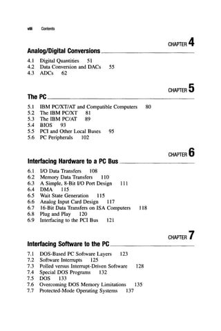
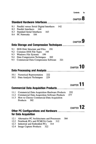
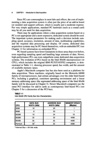
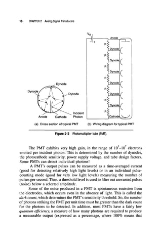
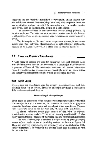
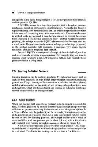
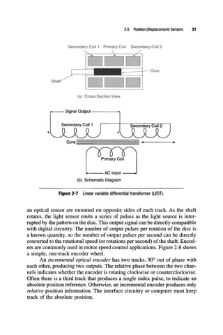
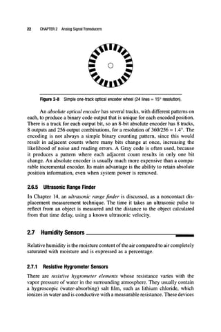
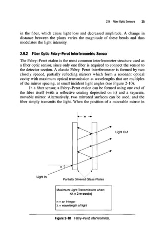
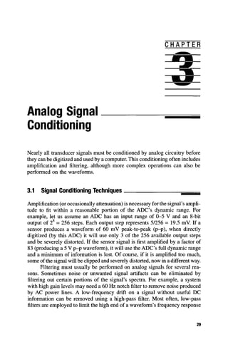
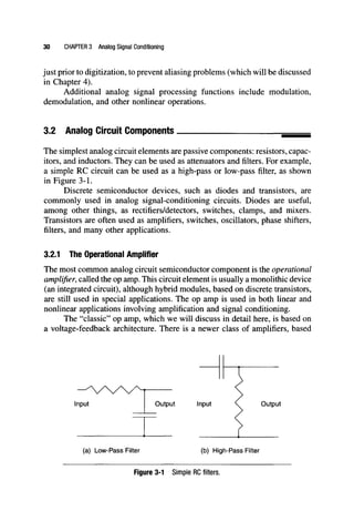
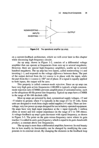
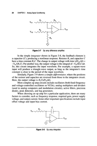
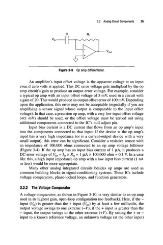
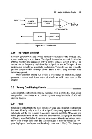
Recently uploaded

Data Acquisition Techniques Using Pcs Second Edition 2nd Edition Howard Austerlitz