Application of OpenSees in Reliability-based Design Optimization of Structures

1| Universidad de La Rioja | 11/07/2014APPLICATION OF OPENSEES IN RBDO OF STRUCTURESOPENSEES DAYS PORTUGAL 2014Luis Celorrio BarraguéDeparmentof MechanicalEngineering–Universidad de La Rioja -Spain

2| Universidad de La Rioja | 11/07/2014
SUMMARY APPLICATION OF OPENSEES IN RELIABILITY BASED DESIGN OPTIMIZATION OF STRUCTURES
RELIABILITY / SENSITIVITY ANALYSIS
RBDO PROBLEM
RBDO METHODS
RBDO WITH OPENSEES
ANALITICAL EXAMPLE
10 BARS TRUSS EXAMPLE
STEELFRAME EXAMPLE
CONCLUSIONS

RELIABILITY / SENSTIVITY ANALYSIS
•Recently, changes in Reliability Modules of OpenSeeshave been carried out. Also some examples, presentations and videos are available in the OpenSeesInternet site.
•New commands provide sensitivity of response with respect to parameters. Also, parameters can be used to map probability distributions to uncertain properties.
•A script-level mechanism for identifying and updating parametershas been added
•Methods to quantify uncertainty are available in OpenSees.
FOSM, FORM, SORM, etc.
Response Sensitivity
Monte Carlo Simulation (Importance Sampling MCS)
System Reliability

4 | Universidad de La Rioja | 11/07/2014
RBDO PROBLEM
 
   
L U L U
t
fi i fi s t P P g P i n
f
X X X
X P
d,μ
d d d μ μ μ
d X P
d μ μ
x
   
   
,
. . , , 0 , 1,...,
min , ,
m XR : vector of random design variables
k dR : vector of deterministic design variables
q PR : vector of random parameters
 Single objective function
 Component level probabilistic constraints
 gi d,X,P 0 Indicates Failure
 X,P Correlated random input variables
where:
The most used formulation of a Reliability Based Design Optimization problem is:

RBDO PROBLEM

RBDO METHODS
Double loop formulations:
Reliability Index Approach (RIA)-based double loop RBDO
Performance Measure Approach (PMA)-based double loop RBDO
Several PMA algorithms: AMV, HMV, HMV+, PMA+ (B.D.Younetal2003, 2005).
Single loop approaches:
SLSV (Single Loop Single Vector)
To Collapse KKT conditions of inner loop as constraints of the outer design loop.
Decoupled (or sequential) approaches:
SORA. (Du and Chen, 2004)

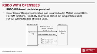
RBDO WITH OPENSEES
•Structural Reliability applications are useful when large structures supporting extreme actions are considered. These extreme actions are wind loads, seismic ground motions or wave loads.
•Then, nonlinear structural behavior must be considered. Also dynamic analysis is necessary when load are time variant. Because that an advanced finite element analysis software is needed.
•OpenSeesis a powerful software with advanced structural analysis capabilities. Also reliability and sensibility functions have been recently modified. Because that OpenSeesbecomes a powerful FEA tool.
•Here some RBDO problems are solved combining some MATLAB functions with the power of OpenSees. These MATLAB functions were originally integrated with FERUM and forming the RBDO –FERUM toolbox. [1]
[1]L.Celorrio-Barragué,“DevelopmentofaReliability-BasedDesignOptimizationToolboxfortheFERUMSoftware”,
SUM2012,LNAI7520,pp.273–286,2012.Springer-VerlagBerlinHeidelberg2012

RBDO WITH OPENSEES
•RBDO RIA-based double loop method
•Outer loop or Design Optimization loop is carried out in Matlabusing RBDO- FERUM functions. Reliability analysis is carried out in OpenSeesusing FORM. Writing/reading of files is used.
Write RVDATA.tcl
Design Variables,
푑푖푖=1,…,푛
Optimization
Loop
RBDO-FERUM
Call !OpenSeesfile.tcl
Read betas.out
Readgradbetas.out
ReadLSFE.out
OPENSEES
Reliability
Loop

RBDO WITH OPENSEES
•RBDO PMA-based double loop method
•Now, Values of Random Variables are passed to OpenSeesto compute the response and the gradients of the response wrtrandom variables. Optimization loop and the search of MPPIR are computed using RBDO- FERUM. Also files are used as interfaces.
Write VECTORDATA.tcl
Random Variables,
푋푖푖=1,…,푁
Optimization
Loop
Sensitivity
Analysis
Call !OpenSeesfilegrad.tcl
Read RES.out
ReadGRADRES.out
Reliability
Loop
RBDO-FERUM
OPENSEES

ANALYTICAL EXAMPLE
 2.0, i 1, 2, 3. t
i 
To minimize 퐶표푠푡 훍퐗 = 휇푋1 + 휇푋2
Subject to 푃 푔푖 푋 ≤ 0 ≤ Φ −훽푖
푡
, 푖 = 1,2,3
0 ≤ 휇푋1 ≤ 10 ; 0 ≤ 휇푋2 ≤ 10
Where the Limit State Functions are
푔1 퐗 = 푋1
2
푋2 20 − 1
푔2 퐗 = 푋1 + 푋2 − 5 2 30 + 푋1 + 푋2 − 12 2 120 − 1
푔3 퐗 = 80 푋1
2 + 8푋2 + 5 − 1
The distribution of the random variables are:
Initial design: 훍퐗
ퟎ = 5.0, 5.0 푇
Convergence Tolerance of the optimization loop: 10−4
푋1~푁 휇푋1 , 퐶표푉 = 0.12
푋2~푁 휇푋2 , 퐶표푉 = 0.12

ANALYTICAL EXAMPLE
Results obtained using RIA based RBDO.
Design Values at the probabilistic optimum: 휇푋1=3.4163휇푋2=3.1335
Cost Function at the probabilistic optimum: 퐶표푠푡훍퐗=6.5497
Reliability Indexes at the optimum: 훽1=2.0171,훽2=2.0109,훽3=7.7892
Number of Optimization Iterations: 15
Number of LSFEs: 1032. It’s very high. We use very small convergence tolerance(10−4in the external loop). Also, no technique to reduce computational effort has been considered.
Gradients are computed using Direct Differentiation Method (Implicit in OpenSees).

ANALYTICAL EXAMPLE

Classic Example in Structural Optimization.
RBDO Problem: To minimize the weight or volume of the truss subject to reliability constraints in terms of displacements or stresses.

CASE 1.- Linear Elastic Material, Linear Analysis.
RBDO Problem: To minimize the volume of the truss subject to reliability
constraints in terms of the vertical displacement of node 2.
To minimize 푉 퐝, 훍퐗, 훍퐏
Subject to 푃 푔푖 푋 ≤ 0 ≤ Φ −훽푖
푡
, 푖 = 1
5푐푚2 ≤ 휇푋푗 ≤ 75푐푚2; 푗 = 1,2,3
Displacement constraint: Vertical displacement at node 2 is limited
u cm allowed displacement a 푔  2  1 퐝, 퐗, 퐏 = 1 −
푢푦2 퐝, 퐗, 퐏
푢푎
Convergence Tolerance of the optimization algorithm: 10−3

CASE 1.- Linear Elastic Material, Linear Analysis
RANDOM VARIABLES OF THE PROBLEM
Random
Variable
Description
Distribution
type
Mean Value
(initial)
CoV or
Standard
Desviation
Design
Variable
1 X 1A LN 20.0 cm2 CoV = 0.05 X1 
2 X A2 LN 20.0 cm2 CoV = 0.05 X2 
3 X A3 LN 20.0 cm2 CoV = 0.05 X3 
4 X E LN 21000.0 kN/cm2 1050 kN/cm2 -
5 X 1 P LN 100.0 kN 20 kN -
6 X 2 P LN 50.0 kN 2.5 kN -
 X1
 X2
 X3
Mean value of the cross section area in horizontal bars.
Mean value of the cross section area in vertical bars.
Mean value of the cross section area in diagonal bars.

Design Values at the probabilistic optimum:
휇푋1=24.1668푐푚2휇푋2=18.2887푐푚2휇푋3=10.2211푐푚2
Volume of Steel at the probabilistic optimum: 퐶표푠푡훍퐗=68783.08푐푚3
Reliability Index at the optimum: 훽1=3.7000,
Number of Optimization Iterations: 61(very high)
Number of LSFEs: 602. Note that the convergence tolerance is small(10−3). Also, no strategy to reduce computational effort has been considered.
Gradients are computed using DDM (Implicit in OpenSees).
CASE 1.-Linear Elastic Material, Linear Analysis

#######################################################################
# FORM ANALYSIS RESULTS, LIMIT-STATE FUNCTION NUMBER 1 #
# #
# Limit-state function value at start point: ......... 0.80548 #
# Limit-state function value at end point: ........... -1.6552e-006 #
# Number of steps: ................................... 4 #
# Number of g-function evaluations: .................. 10 #
# Reliability index beta: ............................ 3.7 #
# FO approx. probability of failure, pf1: ............ 1.07801e-004 #
# #
# rvtagx* u* alpha gamma delta eta #
# 1 2.342e+001 -5.994e-001 -0.16211 -0.16211 0.16746 -0.10514 #
# 2 1.806e+001 -2.309e-001 -0.06246 -0.06246 0.06337 -0.01752 #
# 3 1.002e+001 -3.629e-001 -0.09809 -0.09809 0.10017 -0.04044 #
# 4 1.993e+004 -1.017e+000 -0.27517 -0.27517 0.29001 -0.29337 #
# 5 1.948e+002 3.465e+000 0.93649 0.93649 -0.34563 -3.00061 #
# 6 5.074e+001 3.188e-001 0.08637 0.08637 -0.08526 -0.02319 #
# #
#######################################################################
FORM Results for the last iteration.

#OPENSEES CODE
probabilityTransformationNataf-print 0
randomNumberGeneratorCStdLib
runImportanceSamplingAnalysistruss10MCSa.out -type responseStatistics-maxNum250000 -targetCOV0.01 -print 0
runImportanceSamplingAnalysistruss10MCSb.out -type failureProbability-maxNum250000 -targetCOV0.01 -print 0
#######################################################################
# SAMPLING ANALYSIS RESULTS, LIMIT-STATE FUNCTION NUMBER 1 #
# #
# Estimated mean: .................................... 0.77538 #
# Estimated standard deviation: ...................... 0.16102 #
# #
#######################################################################
#######################################################################
# SAMPLING ANALYSIS RESULTS, LIMIT-STATE FUNCTION NUMBER 1 #
# #
# Reliability index beta: ............................ 3.7151 #
# Estimated probability of failure pf_sim: ........... 0.00010155 #
# Number of simulations: ............................. 250000 #
# Coefficient of variation (of pf): .................. 0.17007 #
#######################################################################
Sampling Analysis Results, using 250000 simulations.

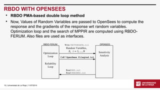
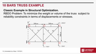
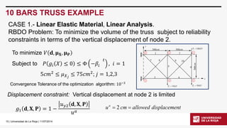
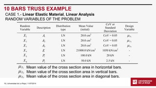
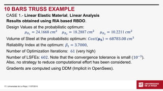
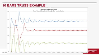
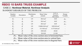
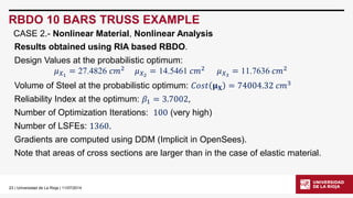
RBDO 10 BARS TRUSS EXAMPLE
uniaxialMaterial Hardening1 $E $fy0.0 [expr$b/(1-$b)*$E]
A random variable is added: fy(elastic limit) ~퐿푁휇=15.5 푘푁푐푚2,퐶표푉=0.05.
$b is the hardening ratio and is considered determinist: set b 0.02
CASE 2.-Nonlinear Material, Nonlinear Analysis

RANDOM VARIABLES OF THE PROBLEM
Random
Variable
Description
Distribution
type
Mean Value
(initial)
CoV or
Standard
Desviation
Design
Variable
1 X 1A LN 20.0 cm2 0.05 X1 
2 X 2A LN 20.0 cm2 0.05 X2 
3 X A3 LN 20.0 cm2 0.05 X3 
4 X E LN 21000.0 kN/cm2 1050 kN/cm2 -
5 X fy LN 15.5 kN/cm2 0.775 kN/cm2 -
6 X 1 P LN 100.0 kN 20 kN -
7 X 2 P LN 50.0 kN 2.5 kN -
 X1
 X2
 X3
Mean value of the cross section area in horizontal bars.
Mean value of the cross section area in vertical bars.
Mean value of the cross section area in diagonal bars.
CASE 2.- Nonlinear Material, Nonlinear Analysis

CASE 2.-Nonlinear Material, Nonlinear Analysis
휇푋1=27.4826푐푚2휇푋2=14.5461푐푚2휇푋3=11.7636푐푚2
Number of LSFEs: 1360.
Note that areas of cross sections are larger than in the case of elastic material.

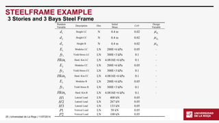
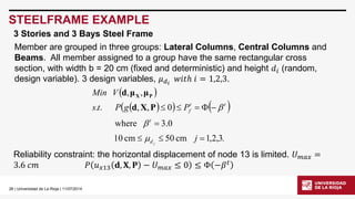
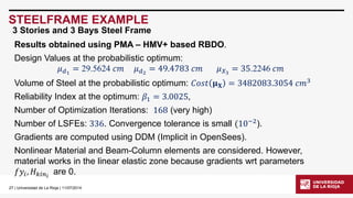
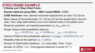
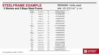
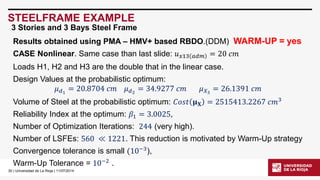
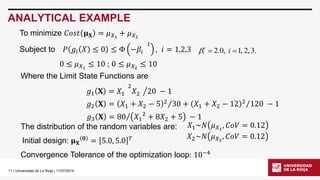
STEELFRAME EXAMPLE
3 Stories and 3 Bays Steel Frame
Modified version of the structural model in the file steelframe.tcl[2] downloaded from OpenSeesforum.
[2]T.HaukaasandM.H.Scott,ShapeSensitivitiesintheReliabilityAnalysisofNonlinearFrameStructures,ComputerandStructures,v.84,15-16,p964-977,2006
1 2 3 1 1 2 2 5 5 5 4 4 4 1 1 1 1 2 2 2 2

STEELFRAME EXAMPLE
Random Variable Description Dist. Initial Mean CoV Design Variable 1d Height LC N 0.4 m 0.02 1d 2d Height CC N 0.4 m 0.02 2d 3d Height B N 0.4 m 0.02 3d 1E Modulus LC LN 200E+6 kPa 0.05 - 1fy Yield Stress LC LN 300E+3 kPa 0.1 - 1Hkin Hard. Kin.LC LN 4.0816E+6 kPa 0.1 - 2E Modulus CC LN 200E+6 kPa 0.05 - 2fy Yield Stress CC LN 300E+3 kPa 0.1 - 2Hkin Hard. Kin.CC LN 4.0816E+6 kPa 0.1 - 3E Modulus B LN 200E+6 kPa 0.05 - 3fy Yield Stress B LN 300E+3 kPa 0.1 - 3Hkin Hard. Kin.B LN 4.0816E+6 kPa 0.1 - 1H Lateral Load LN 400 kN 0.05 2H Lateral Load LN 267 kN 0.05 3H Lateral Load LN 133 kN 0.05 1P Vertical Load LN 50 kN 0.05 2P Vertical Load LN 100 kN 0.05

STEELFRAME EXAMPLE
Member are grouped in three groups: Lateral Columns, Central Columns and
Beams. All member assigned to a group have the same rectangular cross
section, with width b = 20 cm (fixed and deterministic) and height 푑푖 (random,
design variable). 3 design variables, 휇푑푖 푤푖푡ℎ 푖 = 1,2,3.
 
     
j .
s t P g P
Min V
d j
t
t t
f
10 cm 50 cm 1,2,3
where 3.0
. . , , 0
, ,
  

    


d X P 
d μ μX P
Reliability constraint: the horizontal displacement of node 13 is limited. 푈푚푎푥 =
3.6 푐푚 푃 푢푥13 퐝, 퐗, 퐏 − 푈푚푎푥 ≤ 0 ≤ Φ −훽푡

STEELFRAME EXAMPLE
Results obtained using PMA –HMV+ based RBDO.
휇푑1=29.5624푐푚휇푑2=49.4783푐푚휇푋3=35.2246푐푚
Number of LSFEs: 336. Convergence tolerance is small(10−2).
Nonlinear Material and Beam-Column elements are considered. However, material works in the linear elastic zone because gradients wrtparameters 푓푦푖,퐻푘푖푛푖are 0.

STEELFRAME EXAMPLE
Results obtained using PMA –HMV+ based RBDO. (DDM)
CASE Nonlinear. Now, allowed horizontal displacement at node 13 is 20 cm.
Mean Values of Horizontal loads H1, H2 and H3 are the double that in the first case. Then, large deformations occur and material works in the plastic zone.
Response gradients wrtmaterial parameters 푓푦푖,퐻푘푖푛푖are ≠0.
휇푑1=20.8792푐푚휇푑2=34.9506푐푚휇푋3=26.1249푐푚
Number of Optimization Iterations: 256(very high). Time: 1 hour.
Number of LSFEs: 1221. Convergence tolerance is small(10−3).

STEELFRAME EXAMPLE
Random
Variable
Description Dist.
Gradient of Response
wrt Random Variable
1d Height LC N -0.726905589
2 d Height CC N -0.796264509
3 d Height B N -2.066431991
1 E Modulus LC LN -0.000235612
1 fy Yield Stress LC LN -0.021961307
1 Hkin Hard. Kin.LC LN -5.731584490e-6
2 E Modulus CC LN -0.000233264
2 fy Yield Stress CC LN -0.240438494
2 Hkin Hard. Kin.CC LN -0.000403937
3 E Modulus V LN -0.000544820
3 fy Yield Stress V LN -0.393476132
3 Hkin Hard. Kin.V LN -0.000298610
H1 Lateral Load LN 0.0271410404
P1 Vertical Load LN 2.5797303295e-5
P2 Vertical Load LN 1.6692914381e-5
REMARK: Units used
are: 푘푁, 푘푁 푐푚2 푦 푐푚

STEELFRAME EXAMPLE
Results obtained using PMA –HMV+ based RBDO.(DDM) WARM-UP = yes
CASE Nonlinear. Same case than last slide: 푢푥13푎푑푚=20푐푚
Loads H1, H2 and H3 are the double that in the linear case.
휇푑1=20.8704푐푚휇푑2=34.9277푐푚휇푋3=26.1391푐푚
Number of Optimization Iterations: 244(very high).
Number of LSFEs: 560≪1221. This reduction is motivated by Warm-Up strategy
Convergence tolerance is small(10−3),
Warm-Up Tolerance =10−2.

CONCLUSIONS
Sensitivity and Reliability capabilities of OpenSeescan be combined with an optimization tool, such as Optimization Toolbox of Matlabto carry out RBDO.
Double loop RBDO methods have been implemented using OpenSeesand Matlab.
An analytical and two structural examples have been studied.
Complex problems can be solved thanks to advanced structural analysis algorithms implemented in OpenSees.
Computational cost is very high and convergence problems can occur, specially when an increased number of random design variables are considered.
Some special techniques to reduce the computational cost must be added:
Warm up: to start the MPP search in the MPP of the last Iteration.
To use deterministic optimum as initial design

QUESTIONS –COMENTS
THANK YOU
luis.celorrio@unirioja.es
luis.celorrio@gmail.com

Application of OpenSees in Reliability-based Design Optimization of Structures

More Related Content

What's hot

Similar to Application of OpenSees in Reliability-based Design Optimization of Structures

More from openseesdays

Recently uploaded

Application of OpenSees in Reliability-based Design Optimization of Structures