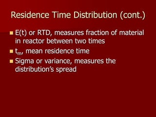
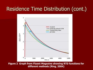
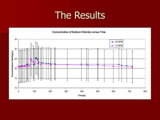
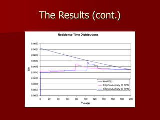
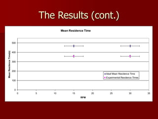
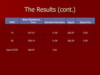
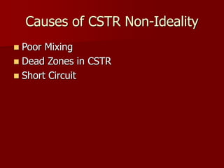
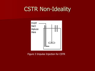
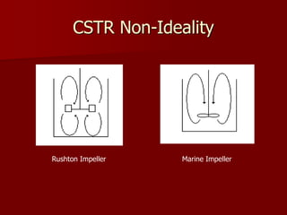
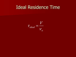
CSTR Ideality
November 29, 2006
By Taryn Herrera
Importance of CSTR Ideality
 Economics
 Design of Reactors
 Higher Conversion of Reactants
CSTR Ideality
 The Experiment
 The Results
 Characterization of Ideality
 Residence Time Distribution Function
 Causes of CSTR Non-Ideality
 Conclusions and Questions
The Experiment
 Characterize the ideality of client’s bench
CSTR reactor
 Operate currently at 30 rpm
 Determine most ideal conditions and make
recommendations
The Experiment (cont.)
 Injection Impulse Step Test
 Sodium Chloride is the Tracer
 Concentration Measurements by
Conductivity
 Different Mixer Speeds
Figure 1 Schematic Diagram for CSTR
Item Description
1 Mixing Point
2 Mixing Point
3 Mixing Point
4 Mixing Points
5
Water Bath Inlet and
Outlet
6
Four Wall Mounted
Baffles
7 Mixer Drive
8 Marine Type Impeller
9 CSTR Vessel
10 Water Bath Vessel
The CSTR Apparatus
Characterization of Ideality
 Ideal Residence Time vs. Mean Residence
Time
 Residence Time is how long material stays
in reactor
 Comparison is done numerically and
graphically
Ideal Residence Time
o
ideal
V

 
Residence Time Distribution
 

end
t
mean
mean dt
t
tE
t
0
)
( 
 

end
t
m dt
t
E
t
t
0
2
)
(
)
(

 



 end
t
dt
t
C
t
C
t
C
t
C
t
E
0
)]
0
(
)
(
[
)
0
(
)
(
)
(
Residence Time Distribution (cont.)
 E(t) or RTD, measures fraction of material
in reactor between two times
 tm, mean residence time
 Sigma or variance, measures the
distribution’s spread
Residence Time Distribution (cont.)
Figure 2 Graph from Fluent Magazine showing RTD functions for
different methods (Ring, 2004)
The Results
Concentration of Sodium Chloride versus Time
10
15
20
25
30
35
0 100 200 300 400 500 600 700 800
Time(s)
Concentration
NaCl(g/L)
30 RPM
15 RPM
The Results (cont.)
Residence Time Distributions
0.0005
0.0007
0.0009
0.0011
0.0013
0.0015
0.0017
0.0019
0.0021
0.0023
0 20 40 60 80 100 120 140 160 180 200
Time(s)
E(t)
Ideal E(t)
E(t) Conductivity 15 RPM
E(t) Conductivity 30 RPM
The Results (cont.)
Mean Residence Time
0
100
200
300
400
500
0 5 10 15 20 25 30 35
RPM
Mean
Residence
Time(s)
Ideal Mean Residence Time
Experimental Residence Times
The Results (cont.)
RPM
Mean Residence
Time Standard Deviation Sigma Sigma/Tau
15 357.57 11.58 206.87 0.58
30 358.14 11.58 206.35 0.58
Ideal CSTR 466.97 5.90
Causes of CSTR Non-Ideality
 Poor Mixing
 Dead Zones in CSTR
 Short Circuit
CSTR Non-Ideality
Figure 3 Impulse Injection for CSTR
CSTR Non-Ideality
Rushton Impeller Marine Impeller
CSTR Non-Ideality

2
ND

 5
3
0
D
N
P
r
PowerNumbe


 Turbulent Mixing
 Done by Baffles and Mixing Speed
 Promotes Better Mixing of Reactants
 Dead Zones Minimized
 Reynolds Number of 4000
Review
 Characterization of Ideality
 Residence Time Distribution Function
 Mean Residence Time vs. Ideal Residence
Time
 CSTR Non-Ideality
Conclusions
 Use Marine Type Impeller
 Promote Turbulence in CSTR
 Choose Wisely the Mixing Points and
Sampling Points
 Use Fluent
 Observe other RTD data
Questions?

CSTR study - RTD for Calciner.ppt

  • 1.
    CSTR Ideality November 29,2006 By Taryn Herrera
  • 2.
    Importance of CSTRIdeality  Economics  Design of Reactors  Higher Conversion of Reactants
  • 3.
    CSTR Ideality  TheExperiment  The Results  Characterization of Ideality  Residence Time Distribution Function  Causes of CSTR Non-Ideality  Conclusions and Questions
  • 4.
    The Experiment  Characterizethe ideality of client’s bench CSTR reactor  Operate currently at 30 rpm  Determine most ideal conditions and make recommendations
  • 5.
    The Experiment (cont.) Injection Impulse Step Test  Sodium Chloride is the Tracer  Concentration Measurements by Conductivity  Different Mixer Speeds
  • 6.
    Figure 1 SchematicDiagram for CSTR Item Description 1 Mixing Point 2 Mixing Point 3 Mixing Point 4 Mixing Points 5 Water Bath Inlet and Outlet 6 Four Wall Mounted Baffles 7 Mixer Drive 8 Marine Type Impeller 9 CSTR Vessel 10 Water Bath Vessel The CSTR Apparatus
  • 7.
    Characterization of Ideality Ideal Residence Time vs. Mean Residence Time  Residence Time is how long material stays in reactor  Comparison is done numerically and graphically
  • 8.
  • 9.
    Residence Time Distribution   end t mean mean dt t tE t 0 ) (     end t m dt t E t t 0 2 ) ( ) (        end t dt t C t C t C t C t E 0 )] 0 ( ) ( [ ) 0 ( ) ( ) (
  • 10.
    Residence Time Distribution(cont.)  E(t) or RTD, measures fraction of material in reactor between two times  tm, mean residence time  Sigma or variance, measures the distribution’s spread
  • 11.
    Residence Time Distribution(cont.) Figure 2 Graph from Fluent Magazine showing RTD functions for different methods (Ring, 2004)
  • 12.
    The Results Concentration ofSodium Chloride versus Time 10 15 20 25 30 35 0 100 200 300 400 500 600 700 800 Time(s) Concentration NaCl(g/L) 30 RPM 15 RPM
  • 13.
    The Results (cont.) ResidenceTime Distributions 0.0005 0.0007 0.0009 0.0011 0.0013 0.0015 0.0017 0.0019 0.0021 0.0023 0 20 40 60 80 100 120 140 160 180 200 Time(s) E(t) Ideal E(t) E(t) Conductivity 15 RPM E(t) Conductivity 30 RPM
  • 14.
    The Results (cont.) MeanResidence Time 0 100 200 300 400 500 0 5 10 15 20 25 30 35 RPM Mean Residence Time(s) Ideal Mean Residence Time Experimental Residence Times
  • 15.
    The Results (cont.) RPM MeanResidence Time Standard Deviation Sigma Sigma/Tau 15 357.57 11.58 206.87 0.58 30 358.14 11.58 206.35 0.58 Ideal CSTR 466.97 5.90
  • 16.
    Causes of CSTRNon-Ideality  Poor Mixing  Dead Zones in CSTR  Short Circuit
  • 17.
    CSTR Non-Ideality Figure 3Impulse Injection for CSTR
  • 18.
  • 19.
    CSTR Non-Ideality  2 ND   5 3 0 D N P r PowerNumbe   Turbulent Mixing  Done by Baffles and Mixing Speed  Promotes Better Mixing of Reactants  Dead Zones Minimized  Reynolds Number of 4000
  • 20.
    Review  Characterization ofIdeality  Residence Time Distribution Function  Mean Residence Time vs. Ideal Residence Time  CSTR Non-Ideality
  • 21.
    Conclusions  Use MarineType Impeller  Promote Turbulence in CSTR  Choose Wisely the Mixing Points and Sampling Points  Use Fluent  Observe other RTD data
  • 22.