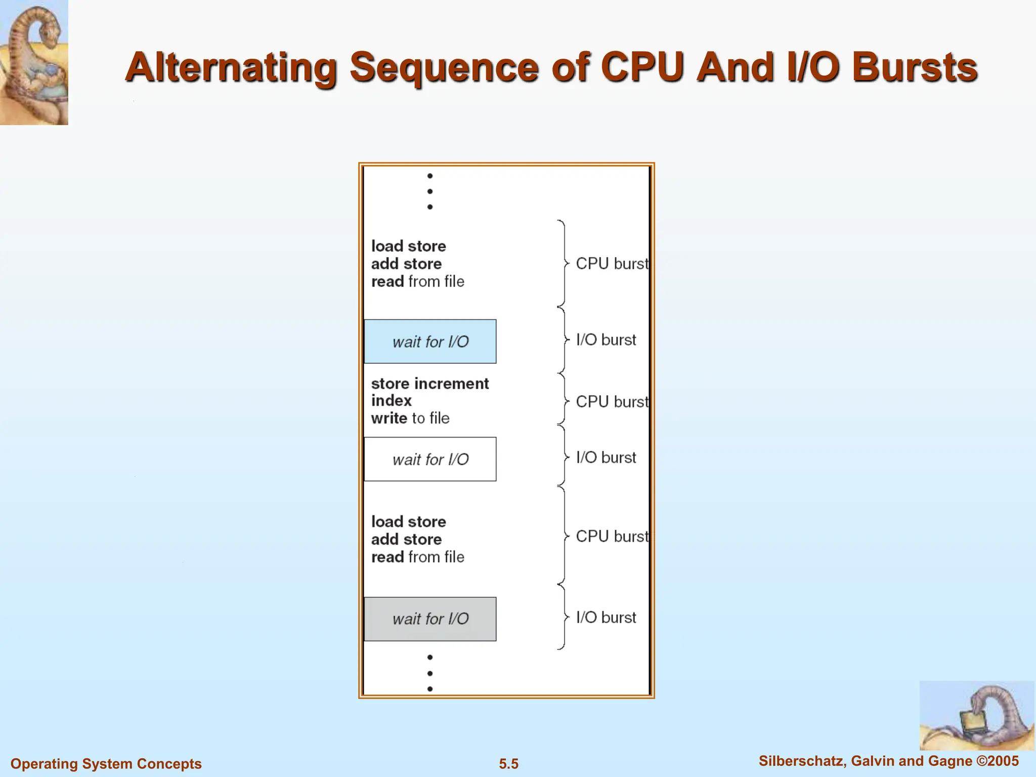
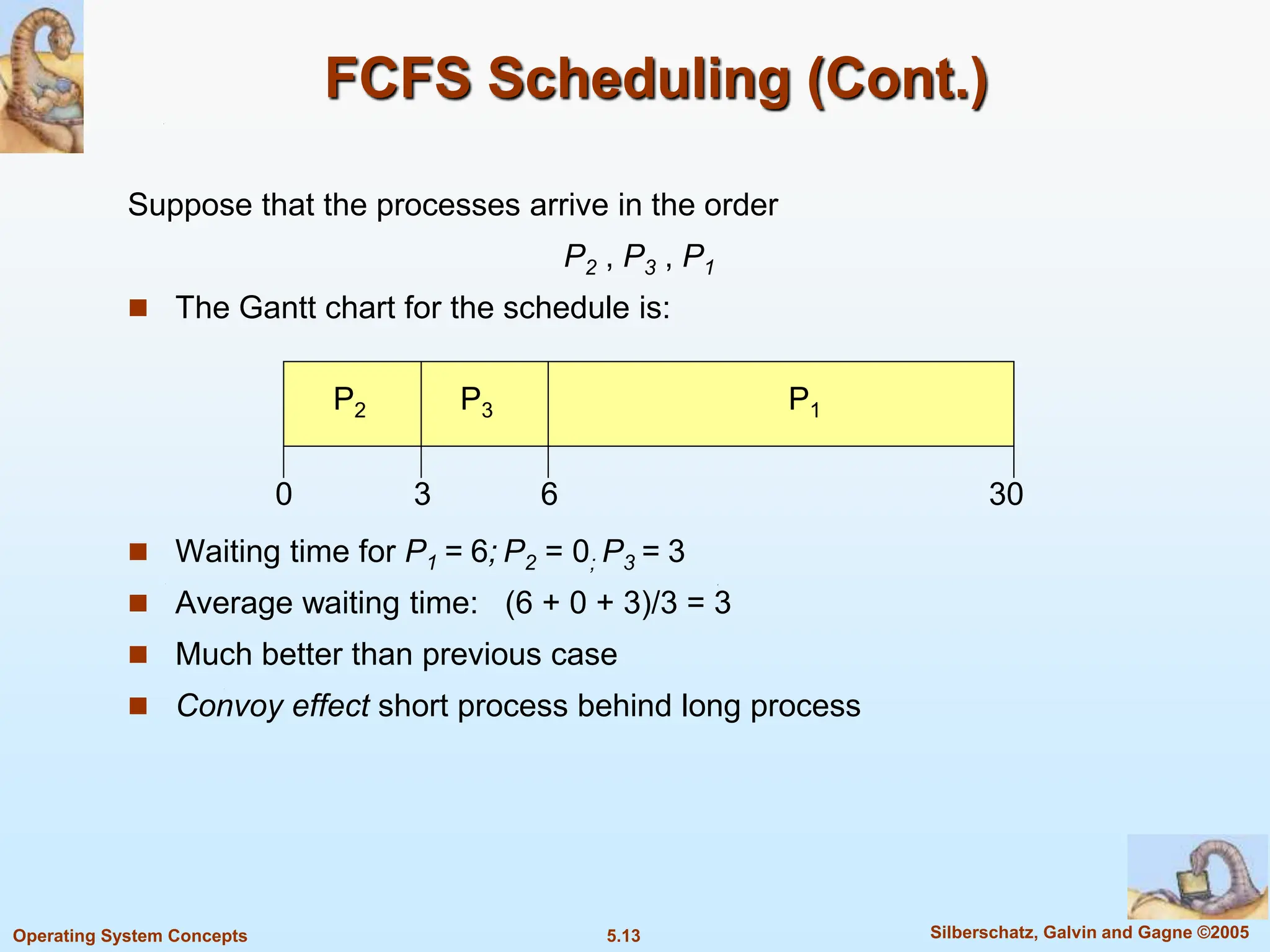
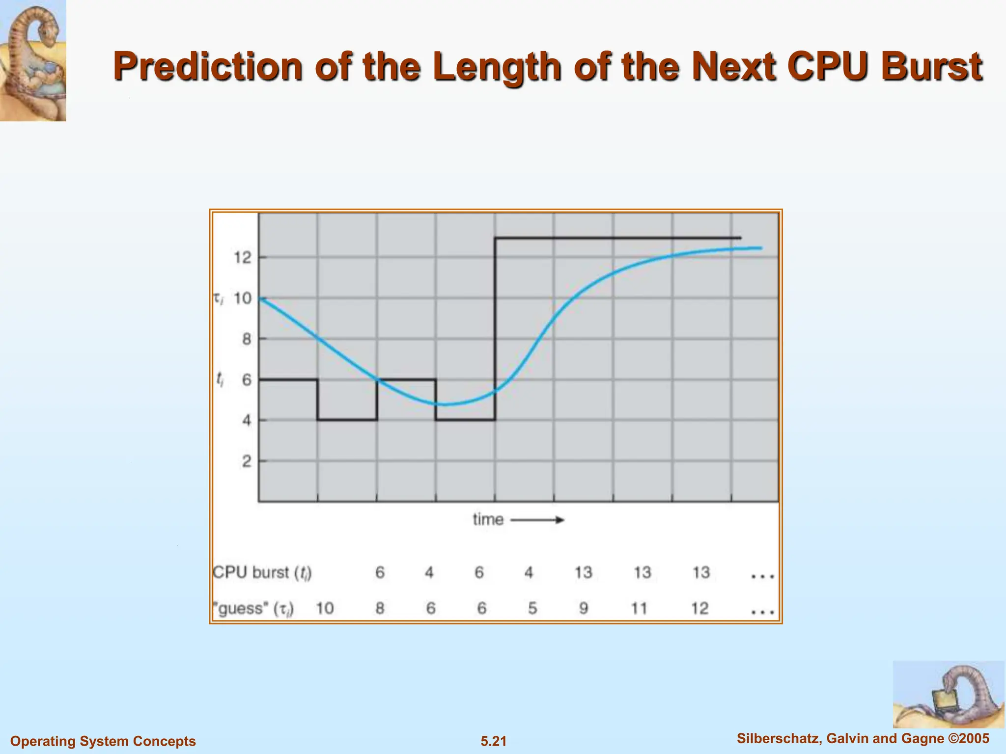
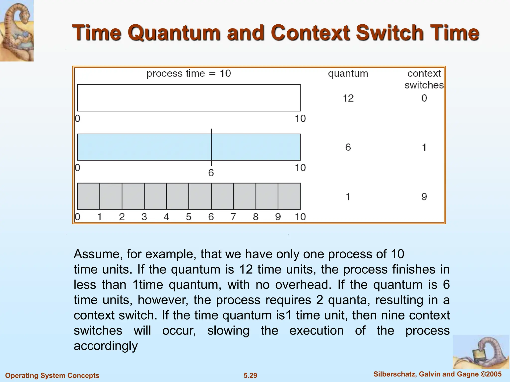
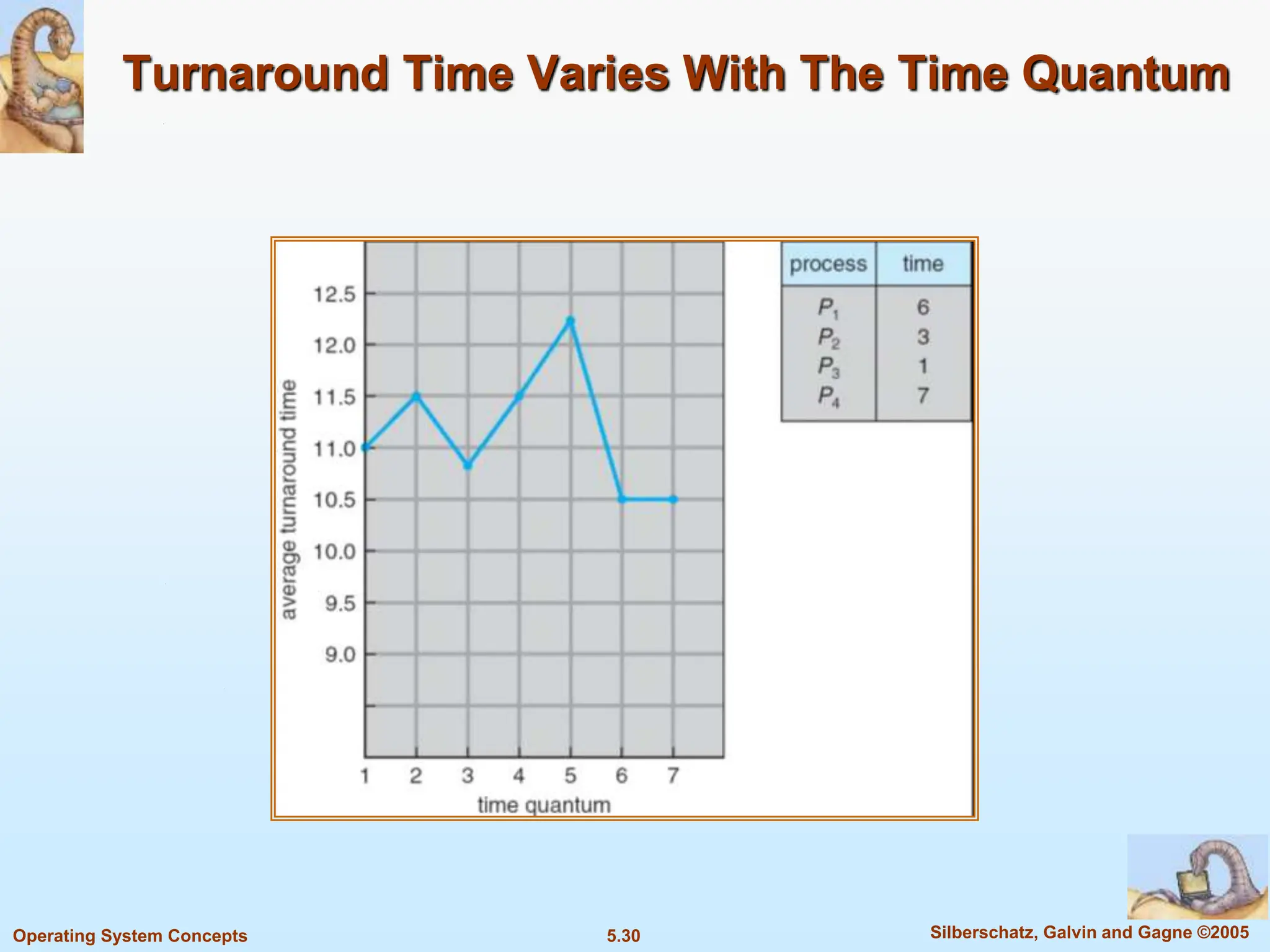
Chapter 5: CPU Scheduling
5.2 Silberschatz, Galvin and Gagne ©2005
Operating System Concepts
Chapter 5: CPU Scheduling
 Basic Concepts
 Scheduling Criteria
 Scheduling Algorithms
 Multiple-Processor Scheduling
 Real-Time Scheduling
 Thread Scheduling
 Operating Systems Examples
 Java Thread Scheduling
 Algorithm Evaluation
5.3 Silberschatz, Galvin and Gagne ©2005
Operating System Concepts
Basic Concepts
 Maximum CPU utilization obtained with multiprogramming
 CPU–I/O Burst Cycle – Process execution consists of a cycle of
CPU execution and I/O wait
 CPU burst distribution
5.4 Silberschatz, Galvin and Gagne ©2005
Operating System Concepts
CPU–I/O Burst Cycle
 The success of CPU scheduling depends on an observed
property of processes:
 process execution consists of a cycle of CPU execution
and I/O wait. Processes alternate between these two
states. Process execution begins with a CPU burst. That is
followed by an I/O burst, which is followed by another
CPU burst, then another I/O burst, and so on. Eventually,
the final CPU burst ends with a system request to terminate
execution
5.5 Silberschatz, Galvin and Gagne ©2005
Operating System Concepts
Alternating Sequence of CPU And I/O Bursts
5.6 Silberschatz, Galvin and Gagne ©2005
Operating System Concepts
 The durations of CPU bursts have been measured extensively.
Although they vary greatly from process to process and from
computer to computer, they tend to have a frequency curve similar
to that shown in Figure on next slide.
 The curve is generally characterized as exponential or
hyperexponential, with a large number of short CPU bursts and a
small number of long CPU bursts.
 An I/O-bound program typically has many short CPU bursts. A
CPU-bound program might have a few long CPU bursts.
 This distribution can be important in the selection of an appropriate
CPU-scheduling algorithm
5.7 Silberschatz, Galvin and Gagne ©2005
Operating System Concepts
Histogram of CPU-burst Times
5.8 Silberschatz, Galvin and Gagne ©2005
Operating System Concepts
CPU Scheduler
 Whenever the CPU becomes idle, the operating
system must select one of the processes in the
ready queue to be executed. The selection
process is carried out by the short-term
scheduler, or CPU scheduler.
5.9 Silberschatz, Galvin and Gagne ©2005
Operating System Concepts
Scheduling Criteria
 CPU utilization – keep the CPU as busy as possible
 Throughput – # of processes that complete their execution per time unit
 Turnaround time – amount of time to execute a particular process
 Waiting time – amount of time a process has been waiting in the ready
queue. The CPU-scheduling algorithm does not affect the amount of time
during which a process executes or does I/O. It affects only the amount of
time that a process spends waiting in the ready queue
 Response time – amount of time it takes from when a request was
submitted until the first response is produced, not output (for time-
sharing environment). In an interactive system, turnaround time may not
be the best criterion. Often, a process can produce some output fairly
early and can continue computing new results while previous results are
being output to the user. Response time, is the time it takes to start
responding, not the time it takes to output the response
5.10 Silberschatz, Galvin and Gagne ©2005
Operating System Concepts
Optimization Criteria
 Max CPU utilization
 Max throughput
 Min turnaround time
 Min waiting time
 Min response time
5.11 Silberschatz, Galvin and Gagne ©2005
Operating System Concepts
First-Come, First-Served (FCFS) Scheduling
 By far the simplest CPU-scheduling algorithm is the first-come, first-
served(FCFS) scheduling algorithm. With this scheme, the
process that requests the CPU first is allocated the CPU first.
 The implementation of the FCFS policy is easily managed with a
FIFO queue. When a process enters the ready queue, its PCB is
linked onto the tail of the queue. When the CPU is free, it is allocated
to the process at the head of the queue. The running process is then
removed from the queue
5.12 Silberschatz, Galvin and Gagne ©2005
Operating System Concepts
First-Come, First-Served (FCFS) Scheduling
Process Burst Time
P1 24
P2 3
P3 3
 Suppose that the processes arrive in the order: P1 , P2 , P3
The Gantt Chart for the schedule is:
 Waiting time for P1 = 0; P2 = 24; P3 = 27
 Average waiting time: (0 + 24 + 27)/3 = 17
P1 P2 P3
24 27 30
0
5.13 Silberschatz, Galvin and Gagne ©2005
Operating System Concepts
FCFS Scheduling (Cont.)
Suppose that the processes arrive in the order
P2 , P3 , P1
 The Gantt chart for the schedule is:
 Waiting time for P1 = 6; P2 = 0; P3 = 3
 Average waiting time: (6 + 0 + 3)/3 = 3
 Much better than previous case
 Convoy effect short process behind long process
P1
P3
P2
6
3 30
0
5.14 Silberschatz, Galvin and Gagne ©2005
Operating System Concepts
FCFS Scheduling (Cont.)
 Note also that the FCFS scheduling algorithm is
nonpreemptive. Once the CPU has been allocated
to a process, that process keeps the CPU until it
releases the CPU, either by terminating or by
requesting I/O.
 The FCFS algorithm is thus particularly
troublesome for time-sharing systems, where it is
important that each user get a share of the CPU at
regular intervals. It would be disastrous to allow
one process to keep the CPU for an extended
period.
5.15 Silberschatz, Galvin and Gagne ©2005
Operating System Concepts
Shortest-Job-First (SJR) Scheduling
 Associate with each process the length of its next CPU burst. Use
these lengths to schedule the process with the shortest time
 When the CPU is available, it is assigned to the process that has
the smallest next CPU burst.
 If the next CPU bursts of two processes are the same, FCFS
scheduling is used to break the tie
5.16 Silberschatz, Galvin and Gagne ©2005
Operating System Concepts
Shortest-Job-First (SJF) Scheduling
 Two schemes:
 nonpreemptive – once CPU given to the process it cannot be
preempted until completes its CPU burst
 preemptive – if a new process arrives with CPU burst length
less than remaining time of current executing process,
preempt. This scheme is know as the
Shortest-Remaining-Time-First (SRTF)
 SJF is optimal – gives minimum average waiting time for a given
set of processes
5.17 Silberschatz, Galvin and Gagne ©2005
Operating System Concepts
Process Arrival Time Burst Time
P1 0.0 7
P2 2.0 4
P3 4.0 1
P4 5.0 4
 SJF (non-preemptive)
 Average waiting time = (0 + 6 + 3 + 7)/4 = 4
Example of Non-Preemptive SJF
P1 P3 P2
7
3 16
0
P4
8 12
5.18 Silberschatz, Galvin and Gagne ©2005
Operating System Concepts
Example of Preemptive SJF
Process Arrival Time Burst Time
P1 0.0 7
P2 2.0 4
P3 4.0 1
P4 5.0 4
 SJF (preemptive)
 Average waiting time = (9 + 1 + 0 +2)/4 = 3
P1 P3
P2
4
2 11
0
P4
5 7
P2 P1
16
5.19 Silberschatz, Galvin and Gagne ©2005
Operating System Concepts
Determining Length of Next CPU Burst
 With short-term scheduling, there is no way to know the
length of the next CPU burst.
 One approach to this problem is to try to approximate SJF
scheduling. We may not know the length of the next CPU
burst, but we may be able to predict its value.
 We expect that the next CPU burst will be similar in length to
the previous ones. By computing an approximation of the
length of the next CPU burst, we can pick the process with
the shortest predicted CPU burst.
 The next CPU burst is generally predicted as an
exponential average of the measured lengths of previous
CPU bursts
5.20 Silberschatz, Galvin and Gagne ©2005
Operating System Concepts
Determining Length of Next CPU Burst
 Can only estimate the length
 Can be done by using the length of previous CPU bursts, using
exponential averaging
:
Define
4.
1
0
,
3.
burst
CPU
next
the
for
value
predicted
2.
burst
CPU
of
lenght
actual
1.
1







n
th
n n
t
  .
1
1 n
n
n t 


 



5.21 Silberschatz, Galvin and Gagne ©2005
Operating System Concepts
Prediction of the Length of the Next CPU Burst
5.22 Silberschatz, Galvin and Gagne ©2005
Operating System Concepts
Examples of Exponential Averaging
  =0
 n+1 = n
 Recent history does not count
  =1
 n+1 =  tn
 Only the actual last CPU burst counts
 If we expand the formula, we get:
n+1 =  tn+(1 - ) tn -1 + …
+(1 -  )j  tn -j + …
+(1 -  )n +1 0
 Since both  and (1 - ) are less than or equal to 1, each
successive term has less weight than its predecessor
5.23 Silberschatz, Galvin and Gagne ©2005
Operating System Concepts
Priority Scheduling
 A priority number (integer) is associated with each process
 The CPU is allocated to the process with the highest priority
(smallest integer  highest priority). Equal-priority processes are
scheduled in FCFS order.
 Preemptive
 nonpreemptive
 When a process arrives at the ready queue, its priority is compared
with the priority of the currently running process. A preemptive
priority scheduling algorithm will preempt the CPU if the priority of
the newly arrived process is higher than the priority of the currently
running process. A nonpreemptive priority scheduling algorithm will
simply put the new process at the head of the ready queue
5.24 Silberschatz, Galvin and Gagne ©2005
Operating System Concepts
Priority Scheduling
 SJF is a priority scheduling where priority is the predicted next CPU
burst time
 Problem  Starvation – low priority processes may never execute
(Rumor has it that when they shut down the IBM 7094 at MIT in
1973, they found a low-priority process that had been submitted in
1967 and had not yet been run.)
 Solution  Aging – as time progresses increase the priority of the
process.
• Aging involves gradually increasing the priority of processes that wait
in the system for a long time. For example, if priorities range from 127
(low) to 0 (high), we could increase the priority of a waiting process by
1 every 15minutes. Eventually, even a process with an initial priority of
127 would have the highest priority in the system and would be
executed. In fact, it would take no more than 32 hours for a priority-127
process to age to a priority-0 process.
5.25 Silberschatz, Galvin and Gagne ©2005
Operating System Concepts
5.26 Silberschatz, Galvin and Gagne ©2005
Operating System Concepts
Round Robin (RR)
 Each process gets a small unit of CPU time (time quantum), usually 10-
100 milliseconds. After this time has elapsed, the process is preempted
and added to the end of the ready queue.
 To implement RR scheduling, we again treat the ready queue as a FIFO
queue of processes. New processes are added to the tail of the ready
queue. The CPU scheduler picks the first process from the ready queue,
sets a timer to interrupt after 1 time quantum, and dispatches the
process.
 One of two things will then happen. The process may have a CPU burst
of less than 1 time quantum. In this case, the process itself will release
the CPU voluntarily. The scheduler will then proceed to the next process
in the ready queue. If the CPU burst of the currently running process is
longer than 1 time quantum, the timer will go off and will cause an
interrupt to the operating system. A context switch will be executed, and
the process will be put at the tail of the ready queue. The CPU scheduler
will then select the next process in the ready queue
5.27 Silberschatz, Galvin and Gagne ©2005
Operating System Concepts
Round Robin (RR)
 Performance
 q large  FCFS
 q small  q must be large with respect to context switch,
otherwise overhead is too high
5.28 Silberschatz, Galvin and Gagne ©2005
Operating System Concepts
Example of RR with Time Quantum = 20
Process Burst Time
P1 53
P2 17
P3 68
P4 24
 The Gantt chart is:
 Typically, higher average turnaround than SJF, but better response
P1 P2 P3 P4 P1 P3 P4 P1 P3 P3
0 20 37 57 77 97 117 121 134 154 162
5.29 Silberschatz, Galvin and Gagne ©2005
Operating System Concepts
Time Quantum and Context Switch Time
Assume, for example, that we have only one process of 10
time units. If the quantum is 12 time units, the process finishes in
less than 1time quantum, with no overhead. If the quantum is 6
time units, however, the process requires 2 quanta, resulting in a
context switch. If the time quantum is1 time unit, then nine context
switches will occur, slowing the execution of the process
accordingly
5.30 Silberschatz, Galvin and Gagne ©2005
Operating System Concepts
Turnaround Time Varies With The Time Quantum
5.31 Silberschatz, Galvin and Gagne ©2005
Operating System Concepts
5.32 Silberschatz, Galvin and Gagne ©2005
Operating System Concepts
Multilevel Queue
 Ready queue is partitioned into separate queues:
foreground (interactive)
background
 Each queue has its own scheduling algorithm
 foreground – RR
 background – FCFS
 Scheduling must be done between the queues
 Fixed priority scheduling; (i.e., serve all from foreground then
from background). Possibility of starvation.
 Time slice – each queue gets a certain amount of CPU time
which it can schedule amongst its processes; i.e., 80% to
foreground in RR, 20% to background in FCFS
5.33 Silberschatz, Galvin and Gagne ©2005
Operating System Concepts
Multilevel Queue Scheduling
5.34 Silberschatz, Galvin and Gagne ©2005
Operating System Concepts
Multilevel Feedback Queue
 A process can move between the various queues; aging can be
implemented this way
 Multilevel-feedback-queue scheduler defined by the following
parameters:
 number of queues
 scheduling algorithms for each queue
 method used to determine when to upgrade a process
 method used to determine when to demote a process
 method used to determine which queue a process will enter
when that process needs service
5.35 Silberschatz, Galvin and Gagne ©2005
Operating System Concepts
Example of Multilevel Feedback Queue
 Three queues:
 Q0 – RR with time quantum 8 milliseconds
 Q1 – RR time quantum 16 milliseconds
 Q2 – FCFS
 Scheduling
 A new job enters queue Q0 which is served FCFS. When it
gains CPU, job receives 8 milliseconds. If it does not finish in 8
milliseconds, job is moved to queue Q1.
 At Q1 job is again served FCFS and receives 16 additional
milliseconds. If it still does not complete, it is preempted and
moved to queue Q2.
5.36 Silberschatz, Galvin and Gagne ©2005
Operating System Concepts
Multilevel Feedback Queues

CPU scheduling are using in operating systems.ppt

  • 1.
    Chapter 5: CPUScheduling
  • 2.
    5.2 Silberschatz, Galvinand Gagne ©2005 Operating System Concepts Chapter 5: CPU Scheduling  Basic Concepts  Scheduling Criteria  Scheduling Algorithms  Multiple-Processor Scheduling  Real-Time Scheduling  Thread Scheduling  Operating Systems Examples  Java Thread Scheduling  Algorithm Evaluation
  • 3.
    5.3 Silberschatz, Galvinand Gagne ©2005 Operating System Concepts Basic Concepts  Maximum CPU utilization obtained with multiprogramming  CPU–I/O Burst Cycle – Process execution consists of a cycle of CPU execution and I/O wait  CPU burst distribution
  • 4.
    5.4 Silberschatz, Galvinand Gagne ©2005 Operating System Concepts CPU–I/O Burst Cycle  The success of CPU scheduling depends on an observed property of processes:  process execution consists of a cycle of CPU execution and I/O wait. Processes alternate between these two states. Process execution begins with a CPU burst. That is followed by an I/O burst, which is followed by another CPU burst, then another I/O burst, and so on. Eventually, the final CPU burst ends with a system request to terminate execution
  • 5.
    5.5 Silberschatz, Galvinand Gagne ©2005 Operating System Concepts Alternating Sequence of CPU And I/O Bursts
  • 6.
    5.6 Silberschatz, Galvinand Gagne ©2005 Operating System Concepts  The durations of CPU bursts have been measured extensively. Although they vary greatly from process to process and from computer to computer, they tend to have a frequency curve similar to that shown in Figure on next slide.  The curve is generally characterized as exponential or hyperexponential, with a large number of short CPU bursts and a small number of long CPU bursts.  An I/O-bound program typically has many short CPU bursts. A CPU-bound program might have a few long CPU bursts.  This distribution can be important in the selection of an appropriate CPU-scheduling algorithm
  • 7.
    5.7 Silberschatz, Galvinand Gagne ©2005 Operating System Concepts Histogram of CPU-burst Times
  • 8.
    5.8 Silberschatz, Galvinand Gagne ©2005 Operating System Concepts CPU Scheduler  Whenever the CPU becomes idle, the operating system must select one of the processes in the ready queue to be executed. The selection process is carried out by the short-term scheduler, or CPU scheduler.
  • 9.
    5.9 Silberschatz, Galvinand Gagne ©2005 Operating System Concepts Scheduling Criteria  CPU utilization – keep the CPU as busy as possible  Throughput – # of processes that complete their execution per time unit  Turnaround time – amount of time to execute a particular process  Waiting time – amount of time a process has been waiting in the ready queue. The CPU-scheduling algorithm does not affect the amount of time during which a process executes or does I/O. It affects only the amount of time that a process spends waiting in the ready queue  Response time – amount of time it takes from when a request was submitted until the first response is produced, not output (for time- sharing environment). In an interactive system, turnaround time may not be the best criterion. Often, a process can produce some output fairly early and can continue computing new results while previous results are being output to the user. Response time, is the time it takes to start responding, not the time it takes to output the response
  • 10.
    5.10 Silberschatz, Galvinand Gagne ©2005 Operating System Concepts Optimization Criteria  Max CPU utilization  Max throughput  Min turnaround time  Min waiting time  Min response time
  • 11.
    5.11 Silberschatz, Galvinand Gagne ©2005 Operating System Concepts First-Come, First-Served (FCFS) Scheduling  By far the simplest CPU-scheduling algorithm is the first-come, first- served(FCFS) scheduling algorithm. With this scheme, the process that requests the CPU first is allocated the CPU first.  The implementation of the FCFS policy is easily managed with a FIFO queue. When a process enters the ready queue, its PCB is linked onto the tail of the queue. When the CPU is free, it is allocated to the process at the head of the queue. The running process is then removed from the queue
  • 12.
    5.12 Silberschatz, Galvinand Gagne ©2005 Operating System Concepts First-Come, First-Served (FCFS) Scheduling Process Burst Time P1 24 P2 3 P3 3  Suppose that the processes arrive in the order: P1 , P2 , P3 The Gantt Chart for the schedule is:  Waiting time for P1 = 0; P2 = 24; P3 = 27  Average waiting time: (0 + 24 + 27)/3 = 17 P1 P2 P3 24 27 30 0
  • 13.
    5.13 Silberschatz, Galvinand Gagne ©2005 Operating System Concepts FCFS Scheduling (Cont.) Suppose that the processes arrive in the order P2 , P3 , P1  The Gantt chart for the schedule is:  Waiting time for P1 = 6; P2 = 0; P3 = 3  Average waiting time: (6 + 0 + 3)/3 = 3  Much better than previous case  Convoy effect short process behind long process P1 P3 P2 6 3 30 0
  • 14.
    5.14 Silberschatz, Galvinand Gagne ©2005 Operating System Concepts FCFS Scheduling (Cont.)  Note also that the FCFS scheduling algorithm is nonpreemptive. Once the CPU has been allocated to a process, that process keeps the CPU until it releases the CPU, either by terminating or by requesting I/O.  The FCFS algorithm is thus particularly troublesome for time-sharing systems, where it is important that each user get a share of the CPU at regular intervals. It would be disastrous to allow one process to keep the CPU for an extended period.
  • 15.
    5.15 Silberschatz, Galvinand Gagne ©2005 Operating System Concepts Shortest-Job-First (SJR) Scheduling  Associate with each process the length of its next CPU burst. Use these lengths to schedule the process with the shortest time  When the CPU is available, it is assigned to the process that has the smallest next CPU burst.  If the next CPU bursts of two processes are the same, FCFS scheduling is used to break the tie
  • 16.
    5.16 Silberschatz, Galvinand Gagne ©2005 Operating System Concepts Shortest-Job-First (SJF) Scheduling  Two schemes:  nonpreemptive – once CPU given to the process it cannot be preempted until completes its CPU burst  preemptive – if a new process arrives with CPU burst length less than remaining time of current executing process, preempt. This scheme is know as the Shortest-Remaining-Time-First (SRTF)  SJF is optimal – gives minimum average waiting time for a given set of processes
  • 17.
    5.17 Silberschatz, Galvinand Gagne ©2005 Operating System Concepts Process Arrival Time Burst Time P1 0.0 7 P2 2.0 4 P3 4.0 1 P4 5.0 4  SJF (non-preemptive)  Average waiting time = (0 + 6 + 3 + 7)/4 = 4 Example of Non-Preemptive SJF P1 P3 P2 7 3 16 0 P4 8 12
  • 18.
    5.18 Silberschatz, Galvinand Gagne ©2005 Operating System Concepts Example of Preemptive SJF Process Arrival Time Burst Time P1 0.0 7 P2 2.0 4 P3 4.0 1 P4 5.0 4  SJF (preemptive)  Average waiting time = (9 + 1 + 0 +2)/4 = 3 P1 P3 P2 4 2 11 0 P4 5 7 P2 P1 16
  • 19.
    5.19 Silberschatz, Galvinand Gagne ©2005 Operating System Concepts Determining Length of Next CPU Burst  With short-term scheduling, there is no way to know the length of the next CPU burst.  One approach to this problem is to try to approximate SJF scheduling. We may not know the length of the next CPU burst, but we may be able to predict its value.  We expect that the next CPU burst will be similar in length to the previous ones. By computing an approximation of the length of the next CPU burst, we can pick the process with the shortest predicted CPU burst.  The next CPU burst is generally predicted as an exponential average of the measured lengths of previous CPU bursts
  • 20.
    5.20 Silberschatz, Galvinand Gagne ©2005 Operating System Concepts Determining Length of Next CPU Burst  Can only estimate the length  Can be done by using the length of previous CPU bursts, using exponential averaging : Define 4. 1 0 , 3. burst CPU next the for value predicted 2. burst CPU of lenght actual 1. 1        n th n n t   . 1 1 n n n t        
  • 21.
    5.21 Silberschatz, Galvinand Gagne ©2005 Operating System Concepts Prediction of the Length of the Next CPU Burst
  • 22.
    5.22 Silberschatz, Galvinand Gagne ©2005 Operating System Concepts Examples of Exponential Averaging   =0  n+1 = n  Recent history does not count   =1  n+1 =  tn  Only the actual last CPU burst counts  If we expand the formula, we get: n+1 =  tn+(1 - ) tn -1 + … +(1 -  )j  tn -j + … +(1 -  )n +1 0  Since both  and (1 - ) are less than or equal to 1, each successive term has less weight than its predecessor
  • 23.
    5.23 Silberschatz, Galvinand Gagne ©2005 Operating System Concepts Priority Scheduling  A priority number (integer) is associated with each process  The CPU is allocated to the process with the highest priority (smallest integer  highest priority). Equal-priority processes are scheduled in FCFS order.  Preemptive  nonpreemptive  When a process arrives at the ready queue, its priority is compared with the priority of the currently running process. A preemptive priority scheduling algorithm will preempt the CPU if the priority of the newly arrived process is higher than the priority of the currently running process. A nonpreemptive priority scheduling algorithm will simply put the new process at the head of the ready queue
  • 24.
    5.24 Silberschatz, Galvinand Gagne ©2005 Operating System Concepts Priority Scheduling  SJF is a priority scheduling where priority is the predicted next CPU burst time  Problem  Starvation – low priority processes may never execute (Rumor has it that when they shut down the IBM 7094 at MIT in 1973, they found a low-priority process that had been submitted in 1967 and had not yet been run.)  Solution  Aging – as time progresses increase the priority of the process. • Aging involves gradually increasing the priority of processes that wait in the system for a long time. For example, if priorities range from 127 (low) to 0 (high), we could increase the priority of a waiting process by 1 every 15minutes. Eventually, even a process with an initial priority of 127 would have the highest priority in the system and would be executed. In fact, it would take no more than 32 hours for a priority-127 process to age to a priority-0 process.
  • 25.
    5.25 Silberschatz, Galvinand Gagne ©2005 Operating System Concepts
  • 26.
    5.26 Silberschatz, Galvinand Gagne ©2005 Operating System Concepts Round Robin (RR)  Each process gets a small unit of CPU time (time quantum), usually 10- 100 milliseconds. After this time has elapsed, the process is preempted and added to the end of the ready queue.  To implement RR scheduling, we again treat the ready queue as a FIFO queue of processes. New processes are added to the tail of the ready queue. The CPU scheduler picks the first process from the ready queue, sets a timer to interrupt after 1 time quantum, and dispatches the process.  One of two things will then happen. The process may have a CPU burst of less than 1 time quantum. In this case, the process itself will release the CPU voluntarily. The scheduler will then proceed to the next process in the ready queue. If the CPU burst of the currently running process is longer than 1 time quantum, the timer will go off and will cause an interrupt to the operating system. A context switch will be executed, and the process will be put at the tail of the ready queue. The CPU scheduler will then select the next process in the ready queue
  • 27.
    5.27 Silberschatz, Galvinand Gagne ©2005 Operating System Concepts Round Robin (RR)  Performance  q large  FCFS  q small  q must be large with respect to context switch, otherwise overhead is too high
  • 28.
    5.28 Silberschatz, Galvinand Gagne ©2005 Operating System Concepts Example of RR with Time Quantum = 20 Process Burst Time P1 53 P2 17 P3 68 P4 24  The Gantt chart is:  Typically, higher average turnaround than SJF, but better response P1 P2 P3 P4 P1 P3 P4 P1 P3 P3 0 20 37 57 77 97 117 121 134 154 162
  • 29.
    5.29 Silberschatz, Galvinand Gagne ©2005 Operating System Concepts Time Quantum and Context Switch Time Assume, for example, that we have only one process of 10 time units. If the quantum is 12 time units, the process finishes in less than 1time quantum, with no overhead. If the quantum is 6 time units, however, the process requires 2 quanta, resulting in a context switch. If the time quantum is1 time unit, then nine context switches will occur, slowing the execution of the process accordingly
  • 30.
    5.30 Silberschatz, Galvinand Gagne ©2005 Operating System Concepts Turnaround Time Varies With The Time Quantum
  • 31.
    5.31 Silberschatz, Galvinand Gagne ©2005 Operating System Concepts
  • 32.
    5.32 Silberschatz, Galvinand Gagne ©2005 Operating System Concepts Multilevel Queue  Ready queue is partitioned into separate queues: foreground (interactive) background  Each queue has its own scheduling algorithm  foreground – RR  background – FCFS  Scheduling must be done between the queues  Fixed priority scheduling; (i.e., serve all from foreground then from background). Possibility of starvation.  Time slice – each queue gets a certain amount of CPU time which it can schedule amongst its processes; i.e., 80% to foreground in RR, 20% to background in FCFS
  • 33.
    5.33 Silberschatz, Galvinand Gagne ©2005 Operating System Concepts Multilevel Queue Scheduling
  • 34.
    5.34 Silberschatz, Galvinand Gagne ©2005 Operating System Concepts Multilevel Feedback Queue  A process can move between the various queues; aging can be implemented this way  Multilevel-feedback-queue scheduler defined by the following parameters:  number of queues  scheduling algorithms for each queue  method used to determine when to upgrade a process  method used to determine when to demote a process  method used to determine which queue a process will enter when that process needs service
  • 35.
    5.35 Silberschatz, Galvinand Gagne ©2005 Operating System Concepts Example of Multilevel Feedback Queue  Three queues:  Q0 – RR with time quantum 8 milliseconds  Q1 – RR time quantum 16 milliseconds  Q2 – FCFS  Scheduling  A new job enters queue Q0 which is served FCFS. When it gains CPU, job receives 8 milliseconds. If it does not finish in 8 milliseconds, job is moved to queue Q1.  At Q1 job is again served FCFS and receives 16 additional milliseconds. If it still does not complete, it is preempted and moved to queue Q2.
  • 36.
    5.36 Silberschatz, Galvinand Gagne ©2005 Operating System Concepts Multilevel Feedback Queues