Coupling to Complex Systems

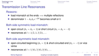
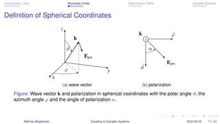
Transmission Lines Stochastic Fields Deterministic Fields Complex Systems
Coupling to Complex Systems
Workshop “You had me at ‘Reverb’!”
at the EMC Europe 2022 in Gothenburg
Dr.-Ing. Mathias Magdowski
Chair for Electromagnetic Compatibility
Institute for Medical Engineering
Otto von Guericke University Magdeburg, Germany
September 5, 2022
License: cb CC BY 4.0 (Attribution, ShareAlike)
Mathias Magdowski Coupling to Complex Systems 2022-09-05 1 / 41

Thanks to the workshop organizers!
Source: https://pixabay.com/photos/thanks-word-letters-scrabble-1804597/

Motivation
Carl Edward Baum in Microwave
Memo No. 3:
“The Microwave Oven Theorem
– All Power to the Chicken”
What is the difference between
a microwave oven and a mode
stirred chamber?
The former cooks chicken, the
later cooks electronics.
How can anyone seriously
consider such a test procedure?
Figure: Carl Edward Baum (1940 – 2010)
Source: http://www.ece.unm.edu/summa/

Change my mind!
Source: https://imgflip.com/i/6sa4e8

Initial Question
All Power to the Chicken?
PInput = PWall + PStirrer + PChicken

Initial Question
PWall = 0

Initial Question
PWall = 0
PStirrer = 0

Initial Question
PWall = 0
PStirrer = 0
PInput = PChicken

Think about it!
Source: https://imgflip.com/i/6sa6a6

Overview
Some Transmission Line Theory
Coupling of Stochastic Fields
Coupling of Deterministic Fields

Hey, can I couple to your transmission line?
Source Radiation "Victim" with cables
Figure: An electromagnetic source affects another electronic device.

Geometry
x
y
z
h
−h
d0
l
k
E
H
Z1 Z2
Figure: Geometry of the line and the exciting plane wave.
Plane wave:
Epw(r) = A0(exx̂ + eyŷ + ezẑ) e−j·(k·r+β)

BLT Equations
▶ after Carl E. Baum, Tom K. Liu and Frederick M. Tesche
▶ developed 1978 at the Kirtland Air Force Base in Albuquerque, New Mexico
(a) C. E. Baum (b) T. K. Liu (c) F. M. Tesche
Figure: Developers of the BLT equations

BLT Equations
Terminal currents:

−I(0)
I(l)

=
1
Zc

(1 − A1) 0
0 (1 − A2)

−A1 ejkl
ejkl −A2
−1
S1
S2


BLT Equations
Terminal currents:

−I(0)
I(l)

=
1
Zc

(1 − A1) 0
0 (1 − A2)

−A1 ejkl
ejkl −A2
−1
S1
S2

Terminal voltages:

U(0)
U(l)

=

(1 + A1) 0
0 (1 + A2)

−A1 ejkl
ejkl −A2
−1
S1
S2


BLT Equations
Terminal currents:

−I(0)
I(l)

=
1
Zc

(1 − A1) 0
0 (1 − A2)

−A1 ejkl
ejkl −A2
−1
S1
S2

Terminal voltages:

U(0)
U(l)

=

(1 + A1) 0
0 (1 + A2)

−A1 ejkl
ejkl −A2
−1
S1
S2

Source term:

S1
S2

= −
1
2



Ee
z
j·(k−kz) − Ut1

1 − ej·(k−kz)l

ejkl

Ee
z
j·(k+kz) + Ut2

1 − e−j·(k+kz)l




Not to be confused with:

Not to be confused with:
Figure: BLT sandwich made with the ingredients bacon, lettuce and tomato.

Auxiliary Variables
Reflection coefficients:
A1 =
Z1 − Zc
Z1 + Zc
A2 =
Z2 − Zc
Z2 + Zc

Auxiliary Variables
A1 =
Z1 − Zc
Z1 + Zc
A2 =
Z2 − Zc
Z2 + Zc
Excitation term:
Ee
z = −j2A0ez sin(kxh)

Auxiliary Variables
A1 =
Z1 − Zc
Z1 + Zc
A2 =
Z2 − Zc
Z2 + Zc
Excitation term:
Ee
z = −j2A0ez sin(kxh)
Transverse voltages:
Ut1 = 2A0
ex
kx
sin(kxh) Ut2 = Ut1 · e−jkzl

Transmission Line Resonances
Reasons:
▶ load mismatch at the ends =⇒ multiple reflections
▶ denominator 1 − A1A2 e−j2kl becomes small or 0

Reasons:
Both-side symmetric load mismatch:
▶ open circuit (A1 = A2 = 1) or short circuit (A1 = A2 = −1)
▶ resonances at l = λ/2, λ, 3/2λ, . . .

Reasons:
Both-side symmetric load mismatch:
▶ open circuit (A1 = A2 = 1) or short circuit (A1 = A2 = −1)
▶ resonances at l = λ/2, λ, 3/2λ, . . .
Both-side asymmetric load mismatch:
▶ open-circuited beginning (A1 = 1) short-circuited end (A2 = −1) or vice
versa
▶ resonances at l = 1/4λ, 3/4λ, 5/4λ, . . .

Which field would you like to have?

Environment: deterministic

EUT: random

EUT: random
Environment: random

EUT: random
Environment: random
EUT: deterministic

Overview

Definition of Spherical Coordinates
x
y
z
k
Epw
φ
ϑ
(a) wave vector
k φ̂
ϑ̂
Epw
α
(b) polarization
Figure: Wave vector k and polarization in spherical coordinates with the polar angle ϑ, the
azimuth angle φ and the angle of polarization α.

Analytical Averaging Procedure
Integration over the full solid angle Ω =
RR
sin ϑ dϑ dφ:
|
D
|I|2
E
| =
1
4π
1
π
1
2π
Z
4π
π
Z
0
2π
Z
0
|I|2
dΩ dα dβ (1)
Usually done for the squared magnitude |I|2
:
▶ equal to I · I∗
▶ real, not complex valued
▶ proportional to the power

Analytical Results for the Load Currents
Transmission line with matched loads:
|
D
|Imatch(0, l)|2
E
| =
1
2

E0h
Zc
2
2 −
sin(2kl)
kl

(2)
Short-circuited transmission line:
|
D
|Ishort(0, l)|2
E
| =
4
1 − cos(2kl)
· |
D
|Imatch(0, l)|2
E
| (3)
Transmission line with general load resistances:
|
D
|I(0)|2
E
| =
(1 + A1)2(1 + A2
2)
1 + A2
1A2
2 − 2 cos(2kl)A1A2
· |
D
|Imatch(0, l)|2
E
| (4)

Example Result of the Stochastic Field Coupling
0.05 0.07 0.1 0.15 0.2 0.3 0.5 0.75 1 1.5 2
10−2
10−1
100
101
102
103
Line length, l/λ
|

|I(0,
l)|
2

|
/
(
E
0
h
/
Z
c
)
2
R1 = R2 = 0
R1 = R2 = 1/10Zc
R1 = R2 = 1/2Zc
R1 = R2 = Zc
R1 = R2 = 2Zc
R1 = R2 = 10Zc
Figure: Mean squared magnitude of the current at the terminals of a transmission line as a
function of the line length. The line has a both-sided symmetric load mismatch.

Comparison with Measurement Results
0.8 1 1.2 1.4 1.6 1.8 2 2.2 2.4 2.6 2.8 3 3.2 3.4 3.6 3.8 4
0
1
2
3
4
Frequency, f (in MHz)
Average
squared
magn.
(in
V
2
)
Measurement
Simulation
Figure: Mean value of the squared magnitude of the coupled voltage at the end of a
205 mm long line as a function of the frequency. (Zc = 230 Ω, R1 = R2 = 50 Ω)

0 5 10 15 20 25 30 35 40
0
0.5
1
1.5
2
Line length, l (in cm)
Average
magnitude
(in
V) Measurement
Simulation
Figure: Mean value of the magnitude of the coupled voltage at the end of the line at
870 MHz as a function of the line length. (Zc = 230 Ω, R1 = R2 = 50 Ω)

0 0.5 1 1.5 2 2.5 3 3.5 4
0
0.2
0.4
0.6
0.8
1
Squared voltage magnitude, U(l) (in V2
)
Cumulative
distribution
function
Measurement
Simulation
Figure: Cumulative distribution function of the squared magnitude of the coupled voltage
at the end of a 322 mm long line at 1.67 GHz (exponential distribution)

Let’s see what we got so far!?
Source: https://imgflip.com/i/6sac6s

Overview

“Average coupling” sounds interesting, but how bad can it get?
Source: https://imgflip.com/i/6sacyn

Maximum Coupling of Deterministic Fields
Deterministic maximum value:
▶ denoted as
x

|I|2
x


▶ coupling from the most effective direction of incidence
▶ not a statistical variable
Finding the most dangerous direction:
▶ second partial derivative test with respect to ϑ, φ and α
▶ numerical simulations
▶ plot of the coupling pattern of the transmission line

Analytical Results for the Maximum Current
x

|I(0)|2
x

 =

A0h · (1 + A1)
Zc
2
·
1
1 − 2A1A2 cos(2kl) + A2
1A2
2
(5)
·
(
4 sin2
(kl) for l ≤ λ
4

1 + |A2| e−2jkl −(1 + |A2|) e−jkl·(1+cos(ϑmax))

2
for l λ
4
Angles of the most effective incident direction:
▶ polarization angle: αmax = −φmax
▶ azimuth angle: φmax = 0 if R2 Zc, φmax = 90◦ if R2 Zc
▶ polar angle:
ϑmax = arccos

atan2(−|A2| sin(2kl),−|A2| cos(2kl)−1)−kl
kl

(6)

Example Result of the Maximum Coupling
0.05 0.07 0.1 0.15 0.2 0.3 0.5 0.75 1 1.5 2
10−1
100
101
102
103
104
Line length, l/λ
x

|I(0,
l)|
2
x

/
(
Eh
/
Z
c
)
2
R1 = R2 = 0
R1 = R2 = 1/10Zc
R1 = R2 = 1/2Zc
R1 = R2 = Zc
R1 = R2 = 2Zc
R1 = R2 = 10Zc
Figure: Deterministic maximum of the squared magnitude of the terminal currents as a
function of the line length. The line has a both-sided symmetric load mismatch.

Discussion of Lifelike Measurement Conditions
Typical immunity test:
▶ illuminate the EUT from only one plane
▶ 4 different directions
▶ 2 orthogonal polarizations
▶ maximum coupling denoted as

2
Reasons:
▶ save costs
▶ directional diagram of a dipole can be assumed for electrically small EUTs

Maximum Coupling From One Plane
0 0.2 0.4 0.6 0.8 1 1.2 1.4 1.6 1.8 2
0
1
2
3
4
5
Line length, l/λ
|I
max,plane
(0)|
2
/
(
Eh
/
Z
c
)
2
x

|I(0)|2
x

 95. percentile 75. percentile
50. percentile 25. percentile 5. percentile
Figure: Lifelike maximum of the squared magnitude of the current at the beginning of a
matched transmission line as a function of the line length.

Losses Caused by the Coupling From One Plane
0 0.2 0.4 0.6 0.8 1 1.2 1.4 1.6 1.8 2
−12
−10
−8
−6
−4
−2
0
Line length, l/λ
|I
max,plane
(0)|
2
↑
|I(0)|
2
↑
(in
dB)
95. percentile
75. percentile
50. percentile
25. percentile
5. percentile
Figure: Ratio between the deterministic maximum and the lifelike maximum of the squared
magnitude of the current at the beginning of a matched transmission line.

Overview

Coupling to Complex Systems

More Related Content

Similar to Coupling to Complex Systems

More from Mathias Magdowski

Recently uploaded

Coupling to Complex Systems