Cosmic rays originate from outside Earth's atmosphere and are detected using scintillators coupled to photomultiplier tubes (PMTs). The authors characterized each PMT by measuring detection rates while varying threshold levels and applied voltages to determine optimal operating parameters. Threshold scans revealed the minimum voltage required to detect particles above noise, while voltage scans showed detection peaks used to set the high voltage for each PMT. Statistical analysis accounted for measurement uncertainties. Data acquisition software converted pulse readings to binary for computer analysis, with words identifying run numbers and detection channels. Overall, adjusting PMT thresholds and voltages improved the quality of cosmic ray energy data collected.

1. Cosmic Ray Detection
Thomas Adams, Cory Oppenheiner
December 5, 2014
Abstract
We measured the operation values of each PMT
using tube characterization scans that allowed
us to read, record, and measure particles passing
through our two scintillators, which allows us to
measure the energy levels of cosmic ray muons
at ground level by setting up and optimizing a
simple Data Acquisition System. Our data is
consistent with our findings and other scientists’
data and experiments
1 Introduction
Cosmic rays are energetic particles that originate
from outside earth’s atmosphere. Being mostly
light, atomic nuclei, cosmic rays are thought
to originate from supernova explosions although
this fact has not been observationally confirmed.
The world’s largest high energy cosmic ray detec-
tor, coving manysquare kilometers in Argentina,
is the Pierre-Auger observatory. Recently, that
telescope has hinted at the possibility that cos-
mic rays originate from highly energetic extra-
galactic sources, not necessarily just supernovae
The main purpose of the Cosmic Ray Detec-
tion experiment was to setup a simple cosmic
ray detection system. We achieved this by us-
ing two scintillating paddles. These two paddles
have Photo Multiplier Tubes or (PMT)s which
are sensors that can sense when light is given
off, due to a high energy particle passing within
the scintillators. These two scintillating paddles
are hooked up to a Data Acquisition System or
(DAQ). However, the main task of our experi-
mental group was to find the best set up of this
system for the collection of cosmic data. Which
includes adjusting threshold levels and the level
of high voltage (HV) applied to each PMT.
1.1 Diagram of our DAQ
The Diagram below shows the wiring of the sys-
tem. Every wire is labeled with it’s delay and
each module is described below.
Figure 1: A scaled picture at the end of the paper
(Figure 8)
2 Characterization Scans
To acquire the best setup for this system we
adjusted the threshold on the Ortec 934 CFD
1

2. card and the amount of HV to the PMT using
the CAEN 1470. To figure out what quantities
these two levels must be set at we had to perform
some tube characterization scans. Once a scan
was completed we knew there would be a double
exponential pattern and that the first plateau
would be the appropriate operational levels of
our scan target PMT.
2.1 Rate vs. Threshold
Threshold: the magnitude or intensity that must
be exceeded for a certain reaction, phenomenon,
result, or condition to occur or be manifested. In
this first graph(Figure 2) which plots Rate with
respect to the voltage you can see that at 50[mV]
the threshold is too low and we are simply ob-
serving noise. At 100[mV] we see a linear trend
that maintains all the way up to 500[mV]. We
decided to not go to any higher thresholds, but
to fill in some of the gaps and took more data
points from 150[mV] - 450[mV] By plotting the
log(Rate) vs. Threshold we were able to see a
plot that has a linearly decreasing slope, roughly
picking where the line crosses the y=0 we chose
a threshold of about 250[mV]. See Figure 2 and
Figure 3. We observed that the threshold values
should be measured and characterized for each
tube.
2.2 Rate vs. Voltage
After finding the proper threshold we decided
to do the voltage scans. We started at -1300[V]
to -2000[V] in 50[V] increments. To control the
amount of time we collected data we used the
CAEN N1145. We set the CAEN N1145 to
count events at 600s per each run. This gave
us a nice double plateau, which will give us the
appropriate operation levels As you can see in
Figure 2: Threshold Plot for tube3.
Figure 3: Threshold Plot for tube4.
2

3. Figure 4, Figure 5, Figure 6 and Figure 7, each
PMT has a different voltage operation level
Figure 4: Voltage Plot for tube1 showing that
tube1 should be set at a voltage of 1700[V].
3 Statistical Uncertainty
During these scans there is always some uncer-
tainty that comes along with it. We used the
Variance Formula to calculate the propagation
of uncertainty of the Log which is the number
of events divided by the total amount of time.
Here is the Variance Formula,
sf =
∂f
∂x
2
s2
x +
∂f
∂t
2
s2
t
Where sx is the error in the number of events
counted, and st is the error in the time. The
variable x is the number of events counted, and
t is the variable for time.
f(x, t) = log
x
t
Figure 5: Voltage Plot for tube2 showing that
tube2 should be set at a voltage of 1790[V].
After plugging in our conditions the equation be-
comes.
sf =
1
xln(10)
2
0 +
−1
600[s]ln(10)
2
0.00052[s]
We assume that there is no error in the events
since there is either an event or not an event.
The error in time we used was half of the smallest
time scale of the CAEN N1145 which is 0.5 [ms].
So, our final uncertainty is equal to:
sf = 3.61912 × 10−7
3.1 Error in Threshold values
The error in the threshold measurements was
dominated by the error in the multimeter mea-
surement. The meter used is a HT39.
Error in DC Voltage Measurment = +/-
(%0.5 of Readback + 2 of the least signifigant
digit)
3

4. Figure 6: Voltage Plot for tube3 showing that
tube3 should be set at a voltage of 1825[V].
3.2 Error in the Readback Voltage vs.
Measured Voltage
The error in the voltage is clearly and solely from
the CAEN 1470 voltage.
Error in the Readback Voltage vs. Mea-
sured Voltage = +/-( %0.02 of Readback +/-
2[Volts] )
4 Analyzer/Reading Data
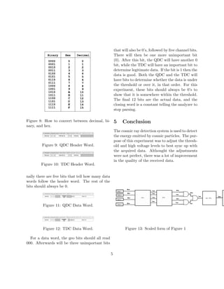
Words
The data taken appears in the following order:
a run count word that tells the run number of
the file, a header word of the QDC to tell hwo
many data words follow (always 16 words) the
data words of the QDC, a header word for the
TDC, the TDC data words, and a closing word
that tells the analyzer to stop parsing.
Figure 7: Voltage Plot for tube4 showing that
tube4 should be set at a voltage of 1720[V].
4.1 Hex to Binary Conversion
The words first appear in hexadecimal, so they
are then converted to binary in order to be read
digitally.On a computer, a word is just a number,
so for the computer it is simply converting one
number to another.
4.2 The Word Make-up
The run count word recalls the run number of
the data. This is used primarily for labeling pur-
poses.
Starting from the left, the first five bits are the
geographical location. This will always be 11111
for this part because our location is constant.
The next three bits denote the kind of word.
A header word will read 010 and a data word
will read 000. For the header word, the next
eight bits denote the crate being used. Both the
TDC and QDC are operating out of crate zero,
so those should be expected to be all 0’s as well.
These are followed by 2 constant zero bits. Fi-
4

5. Figure 8: How to convert between decimal, bi-
nary, and hex.
Figure 9: QDC Header Word.
Figure 10: TDC Header Word.
nally there are five bits that tell how many data
words follow the header word. The rest of the
bits should always be 0.
Figure 11: QDC Data Word.
Figure 12: TDC Data Word.
For a data word, the geo bits should all read
000. Afterwards will be three unimportant bits
that will also be 0’s, followed by five channel bits.
There will then be one more unimportant bit
(0). After this bit, the QDC will have another 0
bit, while the TDC will have an important bit to
determine legitimate data. If the bit is 1 then the
data is good. Both the QDC and the TDC will
have bits to determine whether the data is under
the threshold or over it, in that order. For this
experiment, these bits should always be 0’s to
show that it is somewhere within the threshold.
The final 12 bits are the actual data, and the
closing word is a constant telling the analyzer to
stop parsing.
5 Conclusion
The cosmic ray detection system is used to detect
the energy emitted by cosmic particles. The pur-
pose of this experiment was to adjust the thresh-
old and high voltage levels to best sync up with
the acquired data. Althought the adjustments
were not perfect, there was a lot of improvement
in the quality of the received data.
Figure 13: Scaled form of Figure 1
5