the ppt on control systems good one

1. Introduction to Steady State Error (SSE)
• SSE = Error as time → ∞
• Depends on system type and input
• Measures long-term accuracy

2. Importance of SSE
• Indicates accuracy
• Lower SSE = Better tracking
• Related to system gain and type

3. Static Error Constants
• • Kp, Kv, Ka for step, ramp, parabolic inputs
• • SSE = 1/(1+Kp), etc.
• • Table mapping Type to SSE

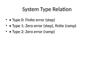
4. System Type Relation
• • Type 0: Finite error (step)
• • Type 1: Zero error (step), finite (ramp)
• • Type 2: Zero error (ramp)

5. Dynamic Error Constants
• • Time-varying behavior
• • More precise than static
• • Used in dynamic systems

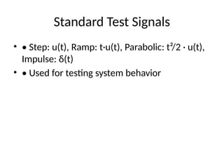
6. Standard Test Signals
• • Step: u(t), Ramp: t·u(t), Parabolic: t²/2 · u(t),
Impulse: δ(t)
• • Used for testing system behavior

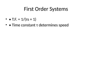
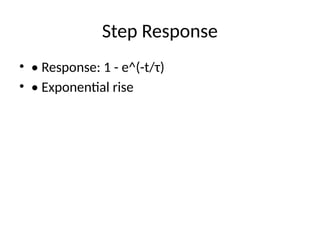
7. First Order Systems
• • T.F. = 1/(τs + 1)
• • Time constant τ determines speed

8. Step Response
• • Response: 1 - e^(-t/τ)
• • Exponential rise

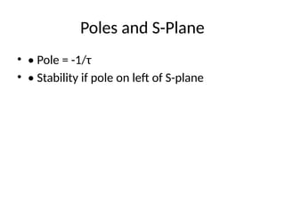
9. Poles and S-Plane
• • Pole = -1/τ
• • Stability if pole on left of S-plane

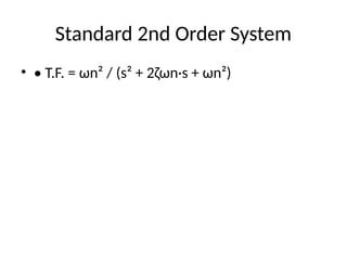
10. Standard 2nd Order System
• • T.F. = ωn² / (s² + 2ζωn·s + ωn²)

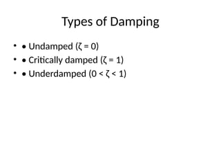
11. Types of Damping
• • Undamped (ζ = 0)
• • Critically damped (ζ = 1)
• • Underdamped (0 < ζ < 1)

12. Time Domain Specs
• • Rise time, Peak time, Settling time,
Overshoot
• • Formulas involve ζ and ωn

13. Pole Locations
• • Poles determine damping and oscillation
• • Example: -2 ± j3 → underdamped

14. Servomotors
• • Used for precise position/speed control
• • Types: AC and DC

15. Comparison
• • AC: low torque, noisy
• • DC: high torque, smooth
• • DC preferred for robotics

16. DC Motor Block Diagram
• • Field-controlled or Armature-controlled
• • Converts electrical → mechanical

17. Torque-Slip
• • AC: nonlinear
• • DC: linear in control region

18. Controller Types
• • P: faster response, small SSE
• • PI: removes SSE, slower
• • PID: fast + zero SSE

19. Transfer Functions
• • PI: Kp + Ki/s
• • PID: Kp + Ki/s + Kd·s

20. Block Diagrams
• • Controller + Plant + Feedback loop
• • Improves system dynamics

21. Stability Definitions
• • Stable: Output bounded
• • Asymptotic: Output → 0
• • Unstable: Output → ∞

22. BIBO Stability
• • Based on pole locations
• • All poles must be left-half S-plane

23. Root Locations
• • Left-half: stable
• • Right-half: unstable
• • Imaginary: marginal

24. Routh-Hurwitz Criterion
• • Use Routh array
• • All +ve signs in first column → stable

25. Special Cases
• • Zero row: use auxiliary polynomial
• • ε substitution if zero in first element

26. Purpose of Root Locus
• • Shows pole movement as gain changes
• • Visual stability analysis

27. Construction Steps
• 1. Open-loop poles/zeros
• 2. Real-axis segments
• 3. Break points
• 4. Asymptotes

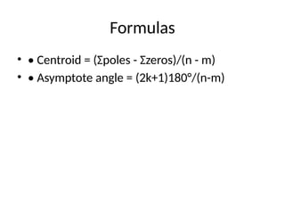
28. Formulas
• • Centroid = (Σpoles - Σzeros)/(n - m)
• • Asymptote angle = (2k+1)180°/(n-m)