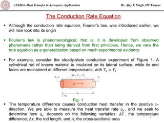
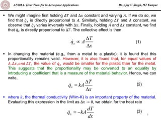
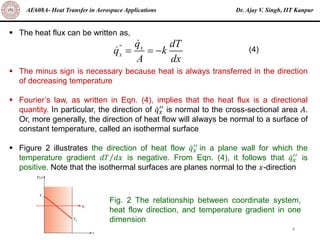
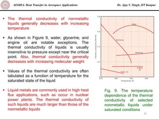
conduction convection djsjjsjshjsjsjskkks

Dr. Ajay V. Singh, IIT Kanpur
AE608A- Heat Transfer in Aerospace Applications
Copyright: The instructor of this course (AE608A) owns the copyright of all the course
materials. The lecture material was distributed only to the students attending the course
AE608A of IIT Kanpur, and should not be distributed in print or through electronic media
without the consent of the instructor. Students can make copies of the course materials
for their use.
Introduction to Conduction
1

2
▪ Although the conduction rate equation, Fourier’s law, was introduced earlier, we
will now look into its origin
▪ Fourier’s law is phenomenological; that is, it is developed from observed
phenomena rather than being derived from first principles. Hence, we view the
rate equation as a generalization based on much experimental evidence
▪ For example, consider the steady-state conduction experiment of Figure 1. A
cylindrical rod of known material is insulated on its lateral surface, while its end
faces are maintained at different temperatures, with 𝑇1 > 𝑇2
▪ The temperature difference causes conduction heat transfer in the positive 𝑥-
direction. We are able to measure the heat transfer rate ሶ
𝑞𝑥, and we seek to
determine how ሶ
𝑞𝑥 depends on the following variables: ∆𝑇 , the temperature
difference; ∆𝑥, the rod length; and 𝐴, the cross-sectional area
The Conduction Rate Equation
Fig. 1

3
▪ We might imagine first holding ∆𝑇 and ∆𝑥 constant and varying 𝐴. If we do so, we
find that ሶ
𝑞𝑥 is directly proportional to 𝐴. Similarly, holding ∆𝑇 and 𝐴 constant, we
observe that ሶ
𝑞𝑥 varies inversely with ∆𝑥. Finally, holding 𝐴 and ∆𝑥 constant, we find
that ሶ
𝑞𝑥 is directly proportional to ∆𝑇. The collective effect is then
▪ In changing the material (e.g., from a metal to a plastic), it is found that this
proportionality remains valid. However, it is also found that, for equal values of
𝐴, ∆𝑥, 𝑎𝑛𝑑 ∆𝑇, the value of ሶ
𝑞𝑥 would be smaller for the plastic than for the metal.
This suggests that the proportionality may be converted to an equality by
introducing a coefficient that is a measure of the material behavior. Hence, we can
write,
▪ where 𝑘, the thermal conductivity (W/m-K) is an important property of the material.
Evaluating this expression in the limit as ∆𝑥 → 0, we obtain for the heat rate
x
T
q A
x



(1)
x
T
q kA
x

=

(2)
x
dT
q kA
dx
= − (3)

4
▪ The heat flux can be written as,
▪ The minus sign is necessary because heat is always transferred in the direction
of decreasing temperature
▪ Fourier’s law, as written in Eqn. (4), implies that the heat flux is a directional
quantity. In particular, the direction of ሶ
𝑞𝑥
′′
is normal to the cross-sectional area 𝐴.
Or, more generally, the direction of heat flow will always be normal to a surface of
constant temperature, called an isothermal surface
▪ Figure 2 illustrates the direction of heat flow ሶ
𝑞𝑥
′′ in a plane wall for which the
temperature gradient Τ
𝑑𝑇 𝑑𝑥 is negative. From Eqn. (4), it follows that ሶ
𝑞𝑥
′′ is
positive. Note that the isothermal surfaces are planes normal to the 𝑥-direction
'' x
x
q dT
q k
A dx
= = − (4)
Fig. 2 The relationship between coordinate system,
heat flow direction, and temperature gradient in one
dimension

5
▪ Recognizing that the heat flux is a vector quantity, we can write a more general
statement of the conduction rate equation (Fourier’s law ) as follows:
▪ where ∇ is the three-dimensional del operator and 𝑇(𝑥, 𝑦, 𝑧) is the scalar
temperature field. It is implicit in Equation (5) that the heat flux vector is in a
direction perpendicular to the isothermal surfaces. An alternative form of Fourier’s
law is therefore,
▪ where ሶ
𝑞𝑛
′′ is the heat flux in a direction 𝑛, which is normal to an isotherm, and ො
𝑛 is
the unit normal vector in that direction
▪ This is illustrated for the two-dimensional case in Figure 3. The heat transfer is
sustained by a temperature gradient along ො
𝑛. Note also that the heat flux vector
can be resolved into components such that, in Cartesian coordinates, the general
expression for ሶ
𝑞′′
is
T T T
ˆ
ˆ ˆ
q k T k i j k
x y z
 
  
 = −  = − + +
 
  
 
(5)
n
T
q q n k n
n

 
= = −

ˆ ˆ (6)
x y z
ˆ
ˆ ˆ
q iq jq kq
   
= + + (7)

6
Fig. 3. The heat flux vector normal to an isotherm in a two-dimensional
coordinate system.
where, from Equation (5), it follows that
▪ Each of these expressions relates the heat flux across a surface to the
temperature gradient in a direction perpendicular to the surface. It is also implicit in
Equation (5) that the medium in which the conduction occurs is isotropic. For such
a medium, the value of the thermal conductivity is independent of the coordinate
direction
▪ Fourier’s law is a vector expression indicating that the heat flux is normal to an
isotherm and in the direction of decreasing temperature. Finally, note that Fourier’s
law applies to all matter, regardless of its state (solid, liquid, or gas)
'' '' ''
x y z
T T T
q k q k q k
x y z
  
= − = − = −
  
(8)

7
The Thermal Properties of Matter
Thermal Conductivity
▪ From Fourier’s law, Equation (8), the thermal conductivity associated with
conduction in the 𝑥-direction is defined as
▪ Similar definitions are associated with thermal conductivities in the y- and z-
directions ( 𝑘𝑦, 𝑘𝑧 ), but for an isotropic material the thermal conductivity is
independent of the direction of transfer, 𝑘𝑥 = 𝑘𝑦 = 𝑘𝑧 ≡ 𝑘
▪ From the foregoing equation, it follows that, for a prescribed temperature gradient,
the conduction heat flux increases with increasing thermal conductivity. In general,
the thermal conductivity of a solid is larger than that of a liquid, which is larger than
that of a gas
▪ As illustrated in Figure 4, the thermal conductivity of a solid may be more than four
orders of magnitude larger than that of a gas. This trend is due largely to
differences in intermolecular spacing for the two states
( )
''
x
x
q
k
T x
= −
 
(9)

8
Fig. 4. Range of thermal conductivity for various states of
matter at normal temperatures and pressure

9
▪ In the modern view of materials, a solid may be comprised of free electrons and
atoms bound in a periodic arrangement called the lattice. Accordingly, transport of
thermal energy may be due to two effects: the migration of free electrons and
lattice vibrational waves
▪ When viewed as a particle-like phenomenon, the lattice vibration quanta are
termed phonons. In pure metals, the electron contribution to conduction heat
transfer dominates, whereas in nonconductors and semiconductors, the phonon
contribution is dominant
▪ Kinetic theory yields the following expression for the thermal conductivity
▪ For conducting materials such as metals, 𝐶 ≡ 𝐶𝑒 is the electron specific heat per
unit volume, ҧ
𝑐 is the mean electron velocity, and 𝜆𝑚𝑓𝑝 ≡ 𝜆𝑒 is the electron mean
free path, which is defined as the average distance traveled by an electron before
it collides with either an imperfection in the material or with a phonon
The Solid State
1
3
mfp
k C c
= (10)

10
▪ In nonconducting solids, 𝐶 ≡ 𝐶𝑝ℎ is the phonon specific heat, ҧ
𝑐 is the average
speed of sound, and 𝜆𝑚𝑓𝑝 ≡ 𝜆𝑝ℎ is the phonon mean free path, which again is
determined by collisions with imperfections or other phonons
▪ In all cases, the thermal conductivity increases as the mean free path of the energy
carriers (electrons or phonons) is increased
▪ When electrons and phonons carry thermal energy leading to conduction heat
transfer in a solid, the thermal conductivity may be expressed as
▪ To a first approximation, 𝑘𝑒 is inversely proportional to the electrical resistivity,
𝜌𝑒. For pure metals, which are of low 𝜌𝑒, 𝑘𝑒 is much larger than 𝑘𝑝ℎ. In contrast, for
alloys, which are of substantially larger 𝜌𝑒, the contribution of 𝑘𝑝ℎ to 𝑘 is no longer
negligible
▪ For nonmetallic solids, 𝑘 is determined primarily by 𝑘𝑝ℎ, which increases as the
frequency of interactions between the atoms and the lattice decreases. The
regularity of the lattice arrangement has an important effect on 𝑘𝑝ℎ, with crystalline
(well-ordered) materials like quartz having a higher thermal conductivity than
amorphous materials like glass
e ph
k k k
= + (11)

11
▪ In fact, for crystalline, nonmetallic solids such as diamond and beryllium oxide, 𝑘𝑝ℎ
can be quite large, exceeding values of 𝑘 associated with good conductors, such
as aluminum
▪ The temperature dependence of 𝑘 is shown in Figure 5 for representative metallic
and nonmetallic solids
Fig. 5

12
The Solid State: Micro- and Nanoscale Effects
▪ In several areas of technology, such as microelectronics,
the material’s characteristic dimensions can be on the
order of micrometers or nanometers, in which case care
must be taken to account for the possible modifications of 𝑘
that can occur as the physical dimensions become small
▪ Cross sections of films of the same material having
thicknesses 𝐿1 and 𝐿2 are shown in Figure 6. Electrons or
phonons that are associated with conduction of thermal
energy are also shown qualitatively. Note that the physical
boundaries of the film act to scatter the energy carriers and
redirect their propagation
▪ For large Τ
𝐿 𝜆𝑚𝑓𝑝 (Figure 6a), the effect of the boundaries
on reducing the average energy carrier path length is
minor, and conduction heat transfer occurs as described for
bulk materials. However, as the film becomes thinner, the
physical boundaries of the material can decrease the
average net distance traveled by the energy carriers, as
shown in Figure 6b Fig. 6

13
▪ The quantity Τ
𝜆𝑚𝑓𝑝 𝐿 is a dimensionless parameter known as the Knudsen number.
Large Knudsen numbers (small Τ
𝐿 𝜆𝑚𝑓𝑝) suggest potentially significant nano- or
microscale effects
▪ Moreover, electrons and phonons moving in the thin 𝑥-direction (representing
conduction in the 𝑥-direction) are affected by the boundaries to a more significant
degree than energy carriers moving in the 𝑦-direction
▪ As such, for films characterized by small Τ
𝐿 𝜆𝑚𝑓𝑝, we find that 𝑘𝑥 < 𝑘𝑦 < 𝑘, where k
is the bulk thermal conductivity of the film material
▪ For Τ
𝐿 𝜆𝑚𝑓𝑝 ≥ 1, the predicted values of 𝑘𝑥 𝑎𝑛𝑑 𝑘𝑦 may be estimated to within 20%
from the following expression
1
3
2
1
3
mfp
x
y mfp
k
k L
k
k L



= −
= −
(12a)
(12b)

14
▪ Equations (12a,b) reveal that the values of 𝑘𝑥 and 𝑘𝑦 are within approximately 5%
of the bulk thermal conductivity if Τ
𝐿 𝜆𝑚𝑓𝑝 > 7 (for 𝑘𝑥) and Τ
𝐿 𝜆𝑚𝑓𝑝 > 4.5 (for 𝑘𝑦)
▪ Values of the mean free path as well as critical film thicknesses below which
microscale effects must be considered, 𝐿𝑐𝑟𝑖𝑡 , are included in Table below for
several materials at 𝑇 ≈ 300 K
▪ For films with 𝜆𝑚𝑓𝑝 < 𝐿 < 𝐿𝑐𝑟𝑖𝑡, 𝑘𝑥 and 𝑘𝑦 are reduced from the bulk value as
indicated in Equations (12a,b)
▪ No general guidelines exist for predicting values of the thermal conductivities for
Τ
𝐿 𝜆𝑚𝑓𝑝 < 1. Note that, in solids, the value of 𝜆𝑚𝑓𝑝 decreases as the temperature
increases

15
▪ In addition to scattering from physical boundaries, as in the case of Figure 6b,
energy carriers may be redirected by chemical dopants embedded within a
material or by grain boundaries that separate individual clusters of material in
otherwise homogeneous matter
▪ Nanostructured materials are chemically identical to their conventional
counterparts but are processed to provide very small grain sizes. This feature
impacts heat transfer by increasing the scattering and reflection of energy carriers
at grain boundaries
▪ Measured values of the thermal
conductivity of a bulk, nanostructured yttria-
stabilized zirconia material are shown in
Figure 7
▪ This particular ceramic is widely used for
insulation purposes in high-temperature
combustion devices. Conduction is
dominated by phonon transfer, and the
mean free path of the phonon energy
carriers is, from Table before, 𝜆𝑚𝑓𝑝 = 25 nm
at 300 K Fig. 7

16
▪ As the grain sizes are reduced to characteristic dimensions less than 25 nm (and
more grain boundaries are introduced in the material per unit volume), significant
reduction of the thermal conductivity occurs
▪ Research on heat transfer in nanostructured materials continues to reveal novel
ways engineers can manipulate the nanostructure to reduce or increase thermal
conductivity

17
▪ The fluid state includes both liquids and gases. Because the intermolecular
spacing is much larger and the motion of the molecules is more random for the
fluid state than for the solid state, thermal energy transport is less effective. The
thermal conductivity of gases and liquids is therefore generally smaller than that of
solids
▪ The effect of temperature, pressure, and chemical species on the thermal
conductivity of a gas may be explained in terms of the kinetic theory of gases
▪ From this theory it is known that the thermal conductivity is directly proportional to
the density of the gas, the mean molecular speed ҧ
𝑐, and the mean free path 𝜆𝑚𝑓𝑝,
which is the average distance traveled by an energy carrier (a molecule) before
experiencing a collision
▪ For an ideal gas, the mean free path may be expressed as,
The Fluid State
1
3
v mfp
k c c
 
 (13)
2
2
B
mfp
k T
d p


= (14)

18
▪ where 𝑘𝐵 is Boltzmann’s constant, 𝑘𝐵 = 1.381 × 10−23
J/K, 𝑑 is the diameter of the
gas molecule, representative values of which are included in Figure 8, and 𝑝 is the
pressure
▪ As expected, the mean free path is small for high pressure or low temperature,
which causes densely packed molecules. The mean free path also depends on the
diameter of the molecule, with larger molecules more likely to experience collisions
than small molecules; in the limiting case of an infinitesimally small molecule, the
molecules cannot collide, resulting in an infinite mean free path
Fig. 8. The temperature dependence of the thermal conductivity of selected gases at
normal pressures. Molecular diameters (d) are in nm. Molecular weights (M) of the
gases are also shown

19
▪ The mean molecular speed, ҧ
𝑐, can be determined from the kinetic theory of gases,
and Equation (13) may ultimately be expressed as
▪ where the parameter 𝛾 is the ratio of specific heats, 𝛾 ≡ Τ
𝑐𝑝 𝑐𝑣 , and 𝑁 is
Avogadro’s number, 𝑁 = 6.022 × 1023
molecules per mol. Equation (15) can be
used to estimate the thermal conductivity of gas, although more accurate models
have been developed
▪ It is important to note that the thermal conductivity is independent of pressure
except in extreme cases as, for example, when conditions approach that of a
perfect vacuum
▪ Therefore, the assumption that 𝑘 is independent of gas pressure for large volumes
of gas is appropriate for the pressures of interest in any engineering problem
▪ Molecular conditions associated with the liquid state are more difficult to describe,
and physical mechanisms for explaining the thermal conductivity are not well
understood
2
9 5
4
v B
c Mk T
k
d N

 
−
= (15)

20
▪ The thermal conductivity of nonmetallic
liquids generally decreases with increasing
temperature
▪ As shown in Figure 9, water, glycerine, and
engine oil are notable exceptions. The
thermal conductivity of liquids is usually
insensitive to pressure except near the critical
point. Also, thermal conductivity generally
decreases with increasing molecular weight
▪ Values of the thermal conductivity are often
tabulated as a function of temperature for the
saturated state of the liquid
▪ Liquid metals are commonly used in high heat
flux applications, such as occur in nuclear
power plants. The thermal conductivity of
such liquids are much larger than those of the
nonmetallic liquids
Fig. 9. The temperature
dependence of the thermal
conductivity of selected
nonmetallic liquids under
saturated conditions

21
The Fluid State: Micro- and Nanoscale Effects
▪ As for the solid state, the bulk thermal conductivity of a fluid may be modified when
the characteristic dimension of the system becomes small, in particular for small
values of Τ
𝐿 𝜆𝑚𝑓𝑝
▪ Similar to the situation of a thin solid film shown in Figure 6b, the molecular mean
free path is restricted when a fluid is constrained by a small physical dimension,
affecting conduction across a thin fluid layer
▪ Mixtures of fluids and solids can also be formulated to tailor the transport
properties of the resulting suspension. For example, nanofluids are base liquids
that are seeded with nanometer-sized solid particles. Their very small size allows
the solid particles to remain suspended within the base liquid for a long time
▪ From the heat transfer perspective, a nanofluid exploits the high thermal
conductivity that is characteristic of most solids, to boost the relatively low thermal
conductivity of base liquids, typical values of which are shown in Figure 9. Typical
nanofluids involve liquid water seeded with nominally spherical nanoparticles of
Al2O3 or CuO

22
▪ In our analysis of heat transfer problems, it will be necessary to use several
properties of matter. These properties are generally referred to as thermophysical
properties and include two distinct categories, transport and thermodynamic
properties
▪ The transport properties include the diffusion rate coefficients such as 𝑘, the
thermal conductivity (for heat transfer), and 𝜈 , the kinematic viscosity (for
momentum transfer)
▪ Thermodynamic properties, on the other hand, pertain to the equilibrium state of a
system. Density (𝜌) and specific heat (𝑐𝑝) are two such properties used extensively
in thermodynamic analysis
▪ The product 𝜌𝑐𝑝 (J/m3-K), commonly termed the volumetric heat capacity,
measures the ability of a material to store thermal energy
▪ Because substances of large density are typically characterized by small specific
heats, many solids and liquids, which are very good energy storage media, have
comparable heat capacities (𝜌𝑐𝑝 > 1 MJ/m3-K)
Other Relevant Properties

23
▪ Because of their very small densities, however, gases are poorly suited for thermal
energy storage (𝜌𝑐𝑝 ≈ 1 kJ/m3-K)
▪ In heat transfer analysis, the ratio of the thermal conductivity to the heat capacity is
an important property termed the thermal diffusivity 𝛼, which has units of m2/s:
▪ It measures the ability of a material to conduct thermal energy relative to its ability
to store thermal energy. Materials of large 𝛼 will respond quickly to changes in their
thermal environment, whereas materials of small 𝛼 will respond more sluggishly,
taking longer to reach a new equilibrium condition
p
k
c


= (16)

24
The Heat Diffusion Equation
▪ A major objective in a conduction analysis is to determine the temperature field in a
medium resulting from conditions imposed on its boundaries
▪ That is, we wish to know the temperature distribution, which represents how
temperature varies with position in the medium. Once this distribution is known, the
conduction heat flux at any point in the medium or on its surface may be computed
from Fourier’s law
▪ We now consider the manner in which the temperature distribution can be
determined. The approach follows the methodology described earlier of applying
the energy conservation requirement
▪ In this case, we define a differential control volume, identify the relevant energy
transfer processes, and introduce the appropriate rate equations. The result is a
differential equation whose solution, for prescribed boundary conditions, provides
the temperature distribution in the medium
▪ Consider a homogeneous medium within which there is no bulk motion (advection)
and the temperature distribution 𝑇(𝑥, 𝑦, 𝑧) is expressed in Cartesian coordinates

25
▪ Let’s define an infinitesimally small (differential) control volume, 𝑑𝑥𝑑𝑦𝑑𝑧, as shown
in Figure 11
▪ Choosing to formulate the first law at an instant of time, the second step is to
consider the energy processes that are relevant to this control volume. In the
absence of motion (or with uniform motion), there are no changes in mechanical
energy and no work being done on the system
Fig. 11. Differential control volume, dx dy dz, for conduction analysis in Cartesian
coordinates

26
▪ Only thermal forms of energy need to be considered. Specifically, if there are
temperature gradients, conduction heat transfer will occur across each of the
control surfaces
▪ The conduction heat rates perpendicular to each of the control surfaces at the x-,
y-, and z-coordinate locations are indicated by the terms ሶ
𝑞𝑥 , ሶ
𝑞𝑦 , and ሶ
𝑞𝑧 ,
respectively. The conduction heat rates at the opposite surfaces can then be
expressed as a Taylor series expansion where, neglecting higher-order terms,
▪ Equation 17a simply states that the 𝑥-component of the heat transfer rate at 𝑥 +
𝑑𝑥 is equal to the value of this component at 𝑥 plus the amount by which it
changes with respect to 𝑥 times 𝑑𝑥
x
x dx x
y
y dy y
z
z dz z
q
q q dx
x
q
q q dy
y
q
q q dz
z
+
+
+

= +


= +


= +

(17a)
(17b)
(17c)

27
▪ Within the medium there may also be an energy source term associated with the
rate of thermal energy generation. This term is represented as,
▪ where ሶ
𝑞′′′ is the rate at which energy is generated per unit volume of the medium
(W/m3)
▪ In addition, changes may occur in the amount of the internal thermal energy stored
by the material in the control volume. If the material is not experiencing a change in
phase, latent energy effects are not pertinent, and the energy storage term may be
expressed as
▪ where 𝜌𝑐𝑝 Τ
𝜕𝑇 𝜕𝑡 is the time rate of change of the sensible (thermal) energy of the
medium per unit volume
▪ Once again it is important to note that the terms ሶ
𝐸𝑔 and ሶ
𝐸𝑠𝑡 represent different
physical processes. The energy generation term is a manifestation of some energy
conversion process involving thermal energy on one hand and some other form of
energy, such as chemical, electrical, or nuclear, on the other
g
E q dx dy dz

=
st p
T
E c dx dy dz
t


=

(18)
(19)

28
▪ The term is positive (a source) if thermal energy is being generated in the material
at the expense of some other energy form; it is negative (a sink) if thermal energy
is being consumed
▪ In contrast, the energy storage term refers to the rate of change of thermal energy
stored by the matter
▪ On a rate basis, the general form of the conservation of energy requirement is,
▪ Hence, recognizing that the conduction rates constitute the energy inflow ሶ
𝐸𝑖𝑛 and
outflow ሶ
𝐸𝑜𝑢𝑡, and substituting, we obtain
▪ Substituting from Equations 17, it follows that
in g out st
E E E E
+ − = (20)
x y z x dx y dy z dz p
T
q q q q dx dy dz q q q c dx dy dz
t

+ + +


+ + + − − − =

(21)
y
x z
x y z x y z p
q
q q T
q q q q dx dy dz q dx q dy q dz c dx dy dz
x y z t


  

+ + + − − − − − − =
   

29
y
x z
p
q
q q T
q dx dy dz dx dy dz c dx dy dz
x y z t


  
 − − − =
   
(22)
▪ The conduction heat rates in an isotropic material may be evaluated from
Fourier’s law,
▪ where each heat flux component of Equation (8) has been multiplied by the
appropriate control surface (differential) area to obtain the heat transfer rate.
Substituting Eqns. (23) into (22) and dividing by (𝑑𝑥𝑑𝑦𝑑𝑧) we have,
x
y
z
T
q k dy dz
x
T
q k dx dz
y
T
q k dx dy
z

= −


= −


= −

(23a)
(23b)
(23c)
p
T T T T
k k k q c
x x y y z z t

 
      
   

+ + + =
 
   
      
   
 
(24)

30
▪ Equation (24) is the general form, in Cartesian coordinates, of the heat diffusion
equation. This equation, often referred to as the heat equation, provides the basic
tool for heat conduction analysis
▪ From its solution, we can obtain the temperature distribution T(x, y, z) as a function
of time
▪ The apparent complexity of this expression should not obscure the fact that it
describes an important physical condition, that is, the conservation of energy
▪ You should have a clear understanding of the physical significance of each term
appearing in the equation. For example, the term Τ
𝜕 𝑘𝜕𝑇/𝜕𝑥 𝜕𝑥 related to the net
conduction heat flux into the control volume for the 𝑥-coordinate direction. That is,
multiplying by 𝑑𝑥,
▪ with similar expressions applying for the fluxes in the y- and z-directions. In words,
the heat equation, Equation (24), therefore states that at any point in the medium
the net rate of energy transfer by conduction into a unit volume plus the volumetric
rate of thermal energy generation must equal the rate of change of thermal energy
stored within the volume
x x dx
T
k dx q q
x x
+
 
 
 
= −
 
 
 
(25)

31
▪ It is often possible to work with simplified versions of Equation (24). For example, if
the thermal conductivity is constant, the heat equation is
▪ Where 𝛼 = Τ
𝑘 𝜌𝑐𝑝 is the thermal diffusivity. Additional simplifications of the general
form of the heat equation are often possible. For example, under steady-state
conditions, there can be no change in the amount of energy storage; hence
Equation (24) reduces to
▪ Moreover, if the heat transfer is one-dimensional (e.g., in the x-direction) and there
is no energy generation, Equation (27) reduces to
2 2 2
2 2 2
p
c
T T T q T
x y z k k t


   
+ + + =
   
2 2 2
2 2 2
1
T T T q T
x y z k t


   
+ + + =
   
(26)
0
T T T
k k k q
x x y y z z
 
     
   

+ + + =
 
   
     
   
 
(27)
0
d dT
k
dx dx
 
=
 
 
(28)

32
▪ The important implication of this result is that, under steady-state, one-dimensional
conditions with no energy generation, the heat flux is a constant in the direction of
transfer ( Τ
𝑑 ሶ
𝑞𝑥
′′ 𝑑𝑥 = 0)
▪ The heat equation may also be expressed in cylindrical and spherical coordinates.
The differential control volumes for these two coordinate systems are shown in
Figures 12 and 13
The Cylindrical Coordinates
Fig. 12. Differential control volume, 𝑑𝑟 ∙ 𝑟𝑑𝜙 ∙ 𝑑𝑧 , for conduction analysis in
cylindrical coordinates (𝑟, 𝜙, 𝑧)

33
▪ When the del operator ∇ of Equation (5) is expressed in cylindrical coordinates, the
general form of the heat flux vector and hence of Fourier’s law is,
▪ Where
▪ are heat flux components in the radial, circumferential, and axial directions,
respectively. Applying an energy balance to the differential control volume of Figure
12, the following general form of the heat equation is obtained:
1
T T T
ˆ
ˆ ˆ
q k T k r z
r r z


 
  
 = −  = − + +
 
  
 
(29)
r
T
q k
r

 = −

k T
q
r



 = −
 z
T
q k
z

 = −

(30)
2
1 1
p
T T T T
kr k k q c
r r r r z z t

 
 
      
   

+ + + =
 
   
      
   
 
(31)

34
The Spherical Coordinates
Fig. 13. Differential control volume, 𝑑𝑟 ∙ 𝑟𝑠𝑖𝑛𝜃𝑑𝜙 ∙ 𝑟𝑑𝜃, for conduction analysis in
spherical coordinates (𝑟, 𝜙, 𝜃)
1 1
T T T
ˆ ˆ
ˆ
q k T k r
r r r sin
 
  
 
  
 = −  = − + +
 
  
 
▪ In spherical coordinates, the general form of the heat flux vector and Fourier’s law
is
▪ where
r
T
q k
r

 = −

k T
q
r



 = −

k T
q
r sin

 

 = −

(32)
(33)

35
▪ Are the heat flux components in the radial, polar, and azimuthal directions,
respectively. Applying an energy balance to the differential control volume of
Figure 13, the following general form of the heat equation is obtained:
▪ Note that the temperature gradient in Fourier’s law must have units of K/m.
Hence, when evaluating the gradient for an angular coordinate, it must be
expressed in terms of the differential change in arc length. For example, the heat
flux component in the circumferential direction of a cylindrical coordinate system is
2
2 2 2 2
1 1 1
p
T T T T
kr k k sin q c
r r r r sin r sin t
 
     
 
      
    
+ + + =
   
 
      
   
 
(34)
and not
k T T
q q k
r
 
 
 
 
= − = −
 

36
Microscale effects
▪ For most practical situations, the heat diffusion equations derived may be used
with confidence
▪ However, these equations are based on Fourier’s law, which does not account for
the finite speed at which thermal information is propagated within the medium by
the various energy carriers
▪ The consequences of the finite propagation speed may be neglected if the heat
transfer events of interest occur over a sufficiently long time scale, Δ𝑡, such that
▪ The heat diffusion equations are invalid for problems where boundary scattering
must be explicitly considered
▪ For example, the temperature distribution within the thin film of Figure 6b cannot
be determined by applying the foregoing heat diffusion equations
1
mfp
c t



37
Boundary and Initial Conditions
▪ To determine the temperature distribution in a medium, it is necessary to solve the
appropriate form of the heat equation
▪ However, such a solution depends on the physical conditions existing at the
boundaries of the medium and, if the situation is time dependent, on conditions
existing in the medium at some initial time
▪ With regard to the boundary conditions, there are several common possibilities
that are simply expressed in mathematical form
▪ Because the heat equation is second order in the spatial coordinates, two
boundary conditions must be expressed for each coordinate needed to describe
the system
▪ Because the equation is first order in time, however, only one condition, termed
the initial condition, must be specified
▪ Three kinds of boundary conditions commonly encountered in heat transfer are
summarized in Table below

38
▪ The conditions are specified at the
surface 𝑥 = 0 for a one-dimensional
system
▪ Heat transfer is in the positive 𝑥-direction
with the temperature distribution, which
may be time dependent, designated as
𝑇(𝑥, 𝑡)
▪ The first condition corresponds to a
situation for which the surface is
maintained at a fixed temperature 𝑇𝑠. It is
commonly termed a Dirichlet condition,
or a boundary condition of the first kind
▪ It is closely approximated, for example,
when the surface is in contact with a
melting solid or a boiling liquid. In both
cases, there is heat transfer at the
surface, while the surface remains at the
temperature of the phase change
process
Boundary conditions for the heat
diffusion equation at the surface (𝑥 = 0)

39
▪ The second condition corresponds to
the existence of a fixed or constant heat
flux at the surface
▪ This heat flux is related to the
temperature gradient at the surface by
Fourier’s law, eq. (8), which may be
expressed as,
▪ It is termed a Neumann condition, or a
boundary condition of the second kind,
and may be realized by bonding a thin
film electric heater to the surface
▪ A special case of this condition
corresponds to the perfectly insulated,
or adiabatic, surface for
which Τ
(𝜕𝑇 𝜕𝑥) 𝑥=0
= 0
( )
0
0 =
'' ''
x s
x
T
q k q
x =

= −


40
▪ The boundary condition of the third
kind corresponds to the existence of
convection heating (or cooling) at the
surface and is obtained from the
surface energy balance

conduction convection djsjjsjshjsjsjskkks

More Related Content

Similar to conduction convection djsjjsjshjsjsjskkks

Recently uploaded

conduction convection djsjjsjshjsjsjskkks